A New Continuum Formulation for Materials--Part II. Some Applications in Fluid Mechanics

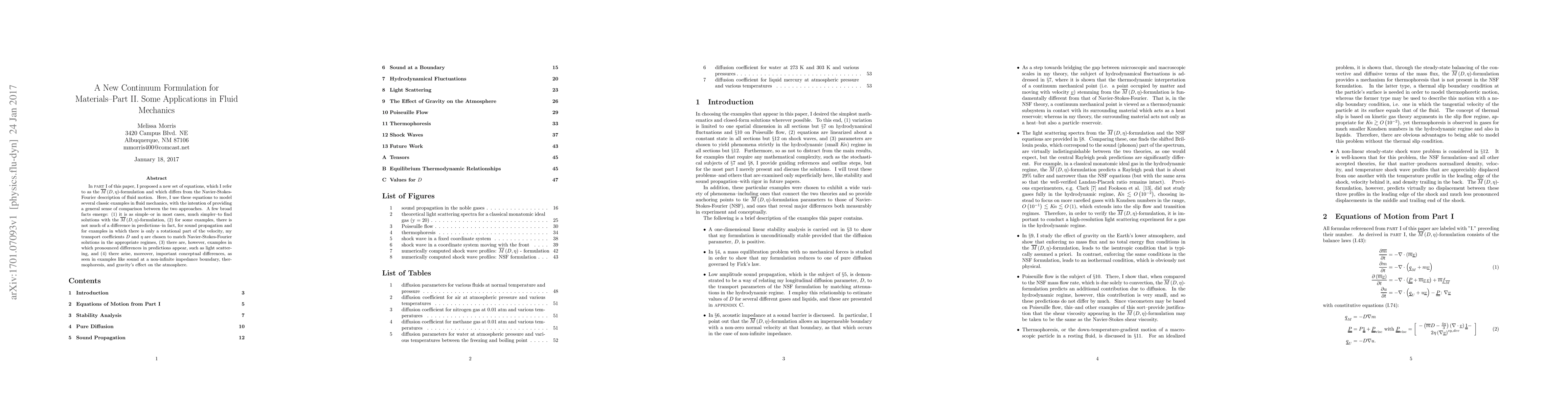
In part I of this paper, I proposed a new set of equations, which I refer to as the M(D,{\eta})-formulation and which differs from the Navier-Stokes-Fourier description of fluid motion. Here, I use these equations to model several classic examples in fluid mechanics, with the intention of providing a general sense of comparison between the two approaches. A few broad facts emerge: (1) it is as simple--or in most cases, much simpler--to find solutions with the M(D,{\eta})-formulation, (2) for some examples, there is not much of a difference in predictions--in fact, for sound propagation and for examples in which there is only a rotational part of the velocity, my transport coefficients D and {\eta} are chosen to match Navier-Stokes-Fourier solutions in the appropriate regimes, (3) there are, however, examples in which pronounced differences in predictions appear, such as light scattering, and (4) there arise, moreover, important conceptual differences, as seen in examples like sound at a non-infinite impedance boundary, thermophoresis, and gravity's effect on the atmosphere.