Discrete Optimization of Statistical Sample Sizes in Simulation by Using the Hierarchical Bootstrap Method

Bootstrap methods are a cornerstone when empirical distributions are unknown or data are scarce, but naïve applications can yield high variance in estimated expectations. This paper tackles a concrete bottleneck in simulation where the inputs Xi are only known through small samples Hi, and the estimator of the form Θ* = E[φ(X1, X2, ..., Xm)] must be computed by repeatedly drawing subsamples from each Hi. In such a setting, the authors propose a discrete optimization of the sample sizes allocated across the hierarchical bootstrap calculation tree. Their goal is to minimize the variance of the final estimator Θ* under a fixed sampling budget, thereby producing more reliable simulation outputs without requiring more primary data.

The breakthrough lies in casting the sample-size allocation problem as a dynamic programming (DP) task over a calculation tree. By introducing backward Bellman-like functions Φv(α, z) and a forward procedure, the method identifies an optimal distribution of sampling effort across the nodes of the tree. This yields a closed-form characterization of the minimal achievable variance, DΘ, as Φk(0, b), and prescribes the optimal vertex-wise sample sizes n*i through a set of discrete, budget-constrained updates. The key innovation is integrating hierarchical bootstrap structure with discrete DP to achieve variance reduction in a principled, computationally tractable way.

How it works at a high level is as follows: for m input variables with samples Hi, one forms L realizations of the subsampled argument vector X(l) by drawing indices from each Hi. The estimator Θ* averages φ(X(l)) over r realizations. The central problem is to minimize the resulting variance DΘ* by allocating the budget b across the k levels (or vertices) of the calculation tree. The authors derive backward recurrence relations for Φv(α, z) using formulas referenced as (27) and (25) in the paper, with the terminal condition Φk(0, b). A forward procedure then computes the optimal sizes ni by solving a constrained minimization (equations (29)–(34) in the paper), ensuring av nv + sum zi ≤ zv and setting α values iteratively. The end result is a concrete recipe for ni that achieves the minimal variance given the budget.

This work matters because it provides a principled, implementable way to make bootstrap-based simulations more efficient when data are scarce or expensive to obtain. By reducing estimator variance without increasing data collection effort, practitioners in engineering, operations research, and risk assessment can achieve more reliable decisions and tighter confidence with the same or lower data costs. The bottom line is that a dynamic-programming framework can transform how we allocate sampling effort inside hierarchical bootstrap computations, delivering measurable variance reductions in complex simulation settings.

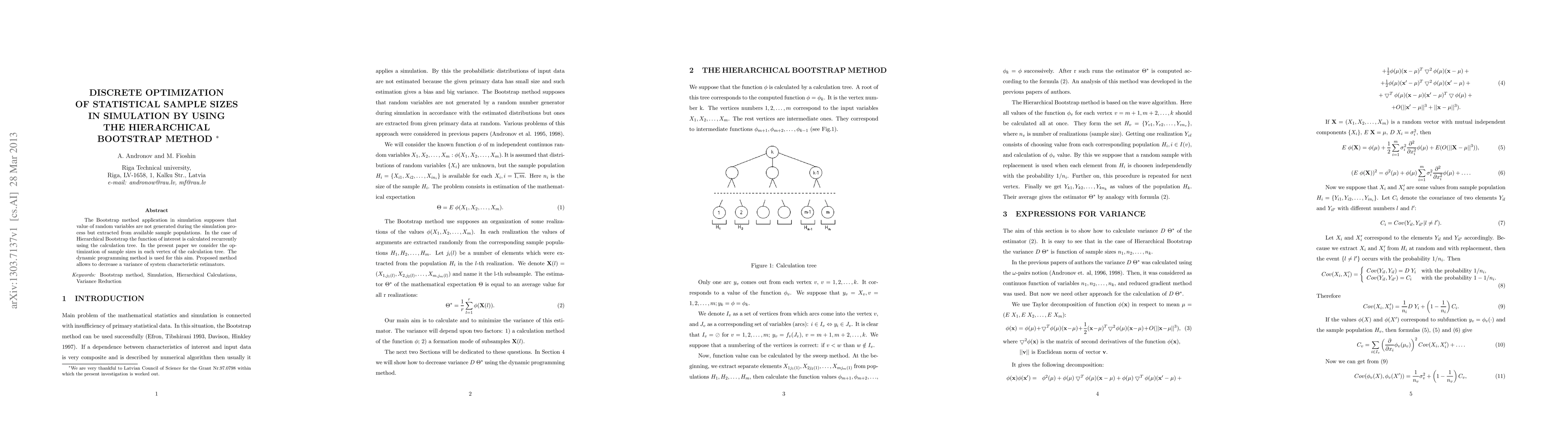
Background The paper addresses a common challenge in simulation and statistics: when the underlying input distributions are unknown and primary data are limited, bootstrap methods are used to resample from available data. In particular, the hierarchical bootstrap builds a calculation tree for a function φ of m independent inputs X1, X2, ..., Xm, each with a finite sample Hi. Realizations of the inputs are constructed by sampling indices ji(l) from each Hi, forming X(l) = (X1, j1(l), X2, j2(l), ..., Xm, jm(l)). The quantity of interest is Θ = E[φ(X1, X2, ..., Xm)], estimated by Θ* = (1/r) ∑l φ(X(l)). The variance of Θ* depends on how subsamples are formed across the tree and on how many samples are allocated at each node, which motivates a discrete optimization of sample sizes to minimize variance.

Problem / Research Question The central question is how to optimally distribute a fixed sampling budget b among the vertices of the hierarchical bootstrap calculation tree to minimize the variance of the estimator Θ*. The problem is modeled within a dynamic programming framework, exploiting the hierarchical, multi-stage structure of the calculation and the fact that sample sizes are discrete. The objective is to derive a minimal-variance estimator and to compute the corresponding optimal per-vertex sample sizes n*i under budget constraints.

Innovation / Contribution The paper advances the methodology by marrying hierarchical bootstrap with discrete dynamic programming. It introduces backward Bellman-type functions Φv(α, z) for the vertices v = 1, 2, ..., k (with k indexing the tree levels) and derives a backward recurrence (formulas akin to (27) and (25)) that computes the minimal achievable variance Φk(0, b). The forward procedure then prescribes how to obtain the optimal per-vertex sample sizes ni by solving a constrained minimization (equations (29)–(34)) subject to av nv + ∑i∈Iv zi ≤ zv, and setting α values through update rules (equation (33)). The result is an explicit methodology to determine ni and the minimal variance DΘ = Φk(0, b).

Methodology / Approach The methodological backbone is as follows:

• Model the hierarchical bootstrap as a calculation tree over m inputs, each with a known sample Hi. The L-th realization uses indices ji(l) to form X(l).
• Define the estimator Θ* as the average of φ over r realizations and aim to minimize its variance by optimizing subsample formation.
• Develop a backward dynamic programming scheme: compute Bellman-style functions Φv(α, z) down the tree, capturing the minimal possible variance given a budget distribution at each node. The terminal value Φk(0, b) represents the minimal variance for the root with total budget b.
• Implement a forward optimization to recover the optimal per-node sample sizes ni, starting from the leaves and proceeding toward the root, while enforcing the budget constraint av nv + ∑ zi ≤ z*v and updating α accordingly.
• Express the final allocation as ni = floor(zi/a_i), delivering discrete, implementable sizes.

Experiments / Evaluation The provided excerpts emphasize the theoretical development and the concrete recurrence relations for computing the optimal variance and sample sizes. Specific numerical experiments, datasets, or empirical comparisons are not included in the excerpts. As such, the evaluation appears to be primarily algorithmic/theoretical, with claims that the dynamic-programming approach yields variance reductions, but detailed experimental validation, benchmark comparisons, or sensitivity analyses are not described in the included text.

Key Results The core result is a principled formula for the minimal estimator variance, DΘ = Φk(0, b), obtained via backward DP over the calculation tree. The optimal per-node sample sizes ni are obtained by a forward DP step that minimizes a sum of square derivative terms under a budget constraint, subject to α updates. The final allocation is discretized by ni = floor(zi/a_i). These results provide a concrete, implementable recipe to reduce the variance of the bootstrap-based estimator under a fixed sampling budget.

Practical Applications This approach is directly applicable to simulations where input uncertainty is managed via bootstrap and where sampling costs are non-trivial. Fields such as reliability engineering, risk analysis, manufacturing simulations, and any domain relying on hierarchical computational models can benefit from a more efficient use of limited data, achieving tighter error bounds without additional data collection.

Limitations & Considerations Several caveats emerge from the excerpt: the method assumes a hierarchical, tree-structured calculation and discrete budgets, which may limit applicability to non-tree dependencies or continuous sampling settings. The computational cost of solving the backward and forward DP, especially for large m or deep trees, is not analyzed here. The approach relies on accurate specification of the a_i constants and the budget b; sensitivity to these inputs, as well as robustness to model misspecification (e.g., dependence among Xi, or non-identical Hi sizes), remains to be explored. Finally, the lack of reported empirical validation in the excerpt leaves open questions about real-world performance across diverse φ functions and input distributions.

In this work, the authors address a common challenge in simulation: how to estimate a complex, real-valued outcome that depends on several uncertain inputs when we can only observe limited historical data. Instead of generating new random inputs from assumed distributions, they rely on the observed data itself (bootstrap) to compute the outcome. But when the computation of the outcome involves a long chain of calculations (a calculation tree), simply resampling once per run can be inefficient and yield high variance. So they propose a hierarchical bootstrap approach that organizes the computation as a tree, where each node represents a subproblem and where you decide how many samples to draw at each node.

The key idea is to minimize the variance of the estimator by optimally allocating a finite sampling budget across the nodes of this tree. They tackle this with dynamic programming: first a backward pass computes Bellman functions that summarize how a small change at one node affects the total variance, and then a forward pass uses those summaries to pick the best number of samples for each node under a total budget. The result is an explicit procedure for choosing sample sizes that minimizes the estimator’s variance, i.e., the variance of the bootstrap estimate of the target expectation Θ = E φ(X1, ..., Xm).

Intuitively, the method treats the simulation as a decision problem: given limited data and a fixed computational budget, where should we spend more sampling effort to get the most precise estimate? By framing this as a hierarchical optimization, the authors provide a principled, algorithmic way to allocate simulation resources across complex, multi-input problems. This matters because it offers a path to more reliable simulation-based conclusions in fields where data are scarce or distributions unknown, such as finance, healthcare, engineering, and operations research, while keeping computation feasible through the dynamic programming decomposition.

Imagine you’re baking a big batch of cookies, and you want to know exactly how tasty they are. But you can’t taste every single cookie, and you only have a small number of chocolate chips and sugar packets from your pantry to test with. You also have a big recipe tree: some parts of the cookie quality depend on the chocolate, some on the sugar, and some on how you mix everything together. You want to decide, given a limited number of tastings (your budget), how many times to sample each ingredient so that your overall guess of the cookie’s tastiness is as accurate as possible.

The researchers came up with a smart plan called dynamic programming. It’s like making a game plan in steps: first figure out, for the last part of the recipe, how many times you should test it given how tight your budget is. Then move up the tree, deciding how to allocate the remaining tests as you go, until you decide exactly how many tastings to do for chocolate, for sugar, and for the mixing step. The magic is that this plan minimizes the chance you’re wrong about how tasty the cookies are, without needing more chips or packets.

What they found is a precise recipe: a set of equations that tell you the best number of samples to take at each step of the recipe, so your final taste estimate has the smallest possible uncertainty under the budget you have. In short, with careful planning, you get more reliable results from the same data.

Why it matters: in real testing—whether designing safer cars, running big service systems, or modeling complex processes—you don’t always have endless data. This method helps scientists and engineers squeeze more reliability out of what they already have, saving time and money while improving decisions.

Bellman functions: a class of functions used in the backward induction step of the dynamic programming approach to minimize variance across a calculation tree — "Bellman functions Φ v(α,z ) for v = 1 , 2,...,k , 0 ≤ α ≤ 1, z = 1 , 2,...,b"\nBootstrap method: a resampling technique where randomness is drawn from the observed data rather than a parametric model — "The Bootstrap method use supposes an organization of some realisations of the values φ(X1,X 2,...,X m)."\nCalculation tree: a hierarchical structure used to organize the evaluation of the function in hierarchical bootstrap — "calculation tree"\nDynamic programming method: an optimization approach to minimize estimator variance by solving sequential subproblems — "The dynamic programming method is used for this aim."\nForward procedure: a phase in the dynamic programming technique that determines the optimal sizes in a forward pass — "forward procedure of dynamic programming technique."\nHierarchical Bootstrap: a bootstrap variant that operates on a hierarchical calculation structure — "Hierarchical Bootstrap"\nHierarchical Calculations: the process of performing hierarchical calculations in the bootstrap framework — "Hierarchical Calculations"\nL-th subsample: a subsample drawn as the l-th sample from the i-th population Hi — "the l-th subsample"\nMathematical expectation: Θ = E φ(X1,X 2,...,X m) — "Θ = E φ(X1,X 2,...,X m)."\nMinimal variance: the smallest possible variance of the estimator; the paper states D∗ Θ ∗ = Φ k(0,b ). — "minimal variance D∗ Θ ∗ = Φ k(0,b )."\nRealization: an instance l where a particular sample is drawn; used with phrases like l-th realization — "l-th realization"\nSubsample: the vector X(l) of drawn values; used with phrases like the l-th subsample — "the l-th subsample"\nVariance reduction: a keyword describing the goal of the method — "Variance Reduction"

• Quantitative validation: how much variance reduction does the DP-based allocation achieve compared with uniform or heuristic subsampling across a range of φ functions and distributions? Provide benchmark results across varying m, n_i, and b.
• Scalability: how does the computational cost grow with the number of inputs m, the tree depth k, and the budget b? Is there a practical ceiling before DP becomes intractable?
• Sensitivity to assumptions: how robust is the method to violations of independence among Xi, different Hi sizes, or mis-specified a_i constants that weight per-node budgets?
• Generalizability: can the framework handle dependent inputs, non-tree calculation structures, or continuous budget spaces rather than discrete b and [z/av] discretization?
• Empirical case studies: are there real-world applications (e.g., engineering reliability, financial risk, or queueing systems) where this method is demonstrated on actual data sets with tangible performance gains?
• Numerical stability: what are the numerical properties of the backward/forward recursions (e.g., sensitivity to rounding, accumulation of error) in large-scale problems?
• Integration with existing bootstrap packages: what are the practical requirements to implement this DP approach in common statistical software, and how does it interface with standard bootstrap variance estimators?
• Extensions to multiple-function objectives: how would the method adapt if several functionals φ1, φ2, ... with different variances must be jointly estimated under a shared budget?

Immediate Applications

• Finance risk simulation: Apply hierarchical bootstrap with dynamic programming to allocate simulation effort across a multi-stage risk model, reducing variance in metrics like VaR or expected shortfall when input distributions are unknown; requires a clearly defined calculation tree φ and available primary data Hi for each input variable.
• Healthcare outcome simulation: Model patient flow or treatment-effect scenarios with limited observational data; use the method to minimize variance in estimated patient-outcome metrics by optimally distributing samples across hierarchical calculation nodes.
• Engineering system reliability: Simulate performance of complex, multi-component systems where outputs depend on a hierarchical calculation tree; benefits include reduced estimator variance and more reliable reliability figures given small data sizes.
• Manufacturing and supply-chain simulations: Multi-stage manufacturing/process models with unknown input distributions; the technique provides principled sample-size allocation across stages to improve estimator precision under budget constraints.
• Data science model evaluation: Multi-metric evaluation pipelines with dependencies across stages; use to obtain more stable estimates of composite scores when data are scarce or expensive to obtain.

Long-Term Applications

• Real-time adaptive simulation with streaming data: Extend the hierarchical bootstrap–DP approach to online settings where sample sizes are adjusted on the fly as data arrive; requires scalable, possibly approximate DP algorithms and fast Bellman-function updates.
• Large-scale, high-dimensional problems: Apply to problems with many inputs and deep calculation trees; needs scalable DP methods, potential approximation schemes, and hardware acceleration to keep computation tractable.
• Policy-driven decision support: Integrate into risk-management or regulatory decision tools where uncertainty in input models is high; requires robust budgeting and policy constraints within the DP optimization framework.