Effective Dimensions of Hierarchical Latent Class Models

Hierarchical latent class (HLC) models are tree-structured Bayesian networks with observed leaves and latent internal nodes. A persistent gap in the field has been the lack of firmly justified model-selection criteria for HLC models, especially given that the standard dimension can mislead when latent variables are present. While practitioners often rely on the BIC score, its theoretical underpinnings weaken in the latent-variable regime, and there is growing evidence that replacing the standard dimension with an effective model dimension can yield better model selection through the BICe or related criteria. However, effective dimensions are notoriously difficult to compute, limiting practical applicability to large models.

The breakthrough of this work is a mathematically precise decomposition that ties the effective dimension of a large regular HLC model to the effective dimensions of smaller, more tractable submodels. Specifically, the authors prove a theorem that expresses the effective dimension of a regular HLC model M with at least two latent nodes as a combination of the effective dimensions of two submodels M1 and M2, obtained by deleting the Z-branch and the X-branch, respectively, and accounting for the parameters they share. This relation reduces the daunting task of computing de(M) to a sequence of computations on smaller HLC or even purely latent-class (LC) models, for which established methods exist.

Beyond this central result, the paper extends the approach to general tree models through a second theorem. This shows that, after pruning latent leaves and decomposing at observed non-leaf nodes, one can express the effective dimension of the whole tree as a sum of effective dimensions of submodels, with irregular submodels regularized without affecting their de. In short, the authors provide a practical, scalable framework to compute effective dimensions for large HLCs and arbitrary trees, enabling the broader use of the BICe/CSe scoring schemes in structure learning.

A key practical upshot is that this decomposition makes it feasible to use effective-dimension penalties in model selection for real-world, large-scale hierarchical latent models. The paper illustrates the point with an empirical example where two competing HLC configurations have the same likelihood on observed data but different effective dimensions; the BIC and BICe scores disagree, highlighting the potential for better decisions when using effective dimensions. The bottom line is that the work equips researchers and practitioners with a principled, scalable tool for more robust model selection and understanding of hierarchical latent structures.

Overall, the contribution advances both theory and practice: it renders the computation of effective dimensions tractable for large HLCs and general trees, and it clarifies how these dimensions interact with model inclusion and regularity to improve scoring-based learning.

Background

Hierarchical latent class (HLC) models are tree-structured Bayesian networks in which leaf nodes are observed and internal nodes are latent. They generalize latent class (LC) models and are used for clustering and structure discovery when hidden factors influence observed data. The paper introduces the notion of the effective dimension de(M) of a Bayesian network M, defined as the regular rank of the Jacobian J_M that maps the model’s parameters to the joint distribution of the observed variables. This rank captures the intrinsic degrees of freedom that actually affect the observed distribution, which can be smaller than the standard dimension ds(M) when latent variables are present. The BIC score, which balances fit and model complexity, can be improved by replacing ds with de in the penalty term, giving the BICe score.

Problem / Research Question

The central challenge is that effective dimensions are hard to compute, especially for large HLC models where latent variables render the Jacobian high-dimensional and algebraically intricate. Although prior work provided complete characterizations for some LC structures and offered computing strategies for LC models, there is no general, scalable method for de(M) in large HLCs or arbitrary trees. The research asks: can we relate the effective dimension of a complex HLC to the effective dimensions of simpler submodels so that computation becomes feasible in practice?

Innovation / Contribution

The paper’s core innovation is a decomposition theorem (Theorem 1) for regular HLC models with two or more latent nodes. By cutting the model along a latent pair (X and its child Z) and constructing two submodels M1 and M2 with appropriate observed sets, the authors show that their effective dimensions combine as de(M) = de(M1) + de(M2) − de_common, where de_common accounts for parameters shared by the submodels. This reduces the problem to computing effective dimensions of smaller HLC or LC models, enabling a recursive solution.

A complementary contribution (Theorem 2) addresses general tree models. After pruning latent leaves and focusing on observed non-leaf nodes, the model can be decomposed at observed nodes into submodels whose effective dimensions add up (with regularization where needed). This provides a systematic way to compute de for any tree model by breaking it down into LC-like pieces and then aggregating results via the main decomposition.

The paper also formalizes a regularity notion to avoid marginally equivalent but parameter-count-expensive representations, and it shows that for regular HLCs, the decomposition preserves regularity, ensuring the computed de is meaningful for model comparison. Importantly, these results connect to practical learning, enabling the use of BICe/CSe scores in learning pipelines.

Methodology / Approach

The method centers on manipulating the parameterization of an HLC model. The authors redefine the joint parameterization to focus on P(X, Z) and then construct two simplified models: M1 (keeping X-branch) and M2 (keeping Z-branch). They analyze the Jacobian matrices J_M, J_M1, and J_M2 and establish correspondences between their columns, proving that the first k0 columns are linearly independent almost everywhere (Claim 1) and that the full column spaces of J_M1 and J_M2 can be spanned by carefully chosen subsets of J_M (Claims 2 and 3). These steps lead to the main equation for de(M).

To illustrate the approach, the authors provide a concrete example with five LC blocks connected through latent nodes, computing the effective dimensions of each LC piece and showing how the overall HLC de emerges from the combination minus shared parameters. They also discuss how to compute LC effective dimensions with existing symbolic-to-numeric strategies (e.g., Geiger et al. 1996) and how the existence of tight bounds (Kocka & Zhang 2002) complements these procedures.

Experiments / Evaluation

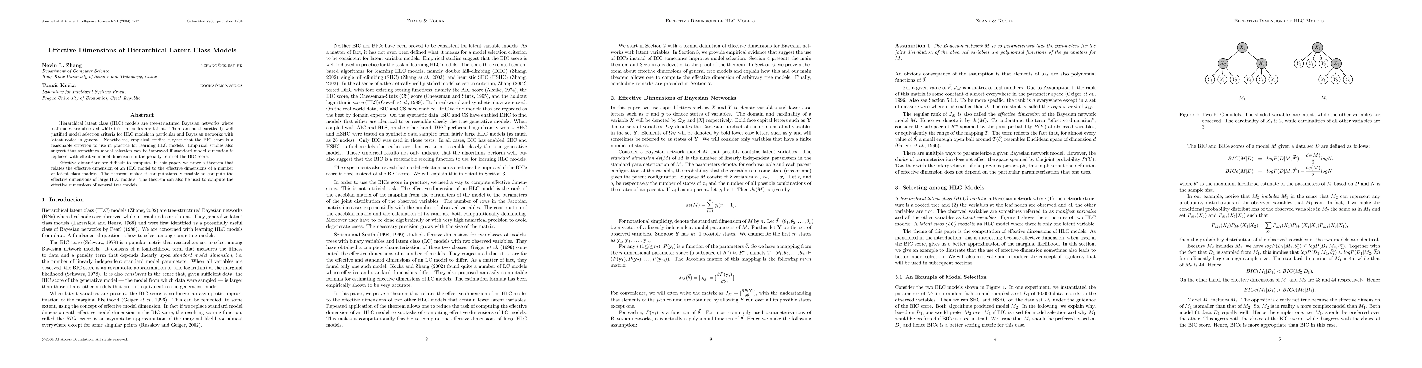
The paper includes an explicit synthetic example contrasting two HLC models M1 and M2. Although M2 includes M1, their standard dimensions differ (ds(M1)=45 vs ds(M2)=44). Their effective dimensions differ as well (de(M1)=43 vs de(M2)=44). This demonstrates that a more complex model in standard terms can have a smaller effective dimension, guiding a preference for the simpler model when using BICe. The example also shows that BIC would favor M2, while BICe favors M1, illustrating the practical impact of using effective dimensions in model selection.

Beyond this example, the authors reference empirical tests on relatively large HLCs (up to 28 nodes) and indicate that the BIC tends to work well in practice, while the BICe/CSe variants can offer improvements in certain cases. The methodology is positioned as enabling scalable computation for larger networks by reducing the problem to LC- and smaller-HLC subproblems.

Key Results

The central theoretical result is Theorem 1: for a regular HLC M with at least two latent nodes, the effective dimension satisfies de(M) = de(M1) + de(M2) − de_common, where M1 and M2 are the submodels obtained by pruning the Z-branch and X-branch, and de_common counts the parameters shared by M1 and M2. This provides a practical, recursive route to de(M).

Theorem 2 extends the idea to general trees: after removing latent leaves and decomposing at observed non-leaf nodes, the effective dimension of the whole tree equals the sum of the effective dimensions of the submodels, with appropriate handling of regu lar (regularized) submodels. Together, these theorems enable decomposing large, structured latent-variable models into LC-like blocks that can be analyzed with existing tools.

Corollaries include the finite, regular search space for regular HLC models with a given set of observed variables, ensuring tractability in model-search settings, and the alignment of de with model inclusion: larger models cannot have smaller effective dimensions than their submodels when inclusion holds, reinforcing the interpretability of de in model comparison.

Practical Applications

The decomposition framework directly supports scalable computation of effective dimensions, which in turn strengthens BICe/CSe as model-selection criteria in structure learning for HLCs and trees. Practically, researchers can:

• Break a large HLC into M1 and M2, compute their de values using LC methods or smaller HLC algorithms, and combine them per the theorems.
• Use existing algorithms (e.g., Geiger et al. 1996) to obtain LC effective dimensions, benefiting from mature tooling.
• Apply the BICe or CSe scores in learning pipelines to potentially improve model selection in domains where latent hierarchies are natural (e.g., bioinformatics, psychology, marketing).

The results also offer theoretical guidance for constructing regular, non-redundant HLC models, since regularity ensures that the decomposition reflects genuine degrees of freedom rather than artifacts of parameterization.

Limitations & Considerations

The core results rely on regular HLC models and on the assumption that the parameterization yields polynomial functions of the joint distribution of observed variables (Assumption 1). The effective dimension is a regular rank, which holds almost everywhere but may be ill-defined at measure-zero singularities; in practice these degeneracies must be treated with care.

Computing de(M) ultimately reduces to calculating de for LC blocks, which themselves can be computationally intensive for very large LC families or highly parameterized state spaces. While the theorems provide a principled reduction, the practical cost remains tied to solving Jacobians and performing rank determinations, particularly as variable cardinalities grow.

The regularization step in handling irregular submodels is well-motivated but may introduce additional overhead or choices that could affect reproducibility across implementations. Moreover, while the decomposition is theoretically sound, real-world models may violate the assumptions (e.g., non-regular structures) or require ad hoc preprocessing to ensure regularity.

Finally, while the framework supports general trees, its empirical performance hinges on the efficiency of LC-decomposition routines and the availability of robust numerical tools for rank estimation on polynomial-parameterized Jacobians. These dependencies suggest avenues for further optimization and benchmarking across diverse domains.

Hidden, hierarchical structures are common in data: some variables we can observe directly, while many others are latent and influence what we see. When we try to learn such models from data, a standard penalty for complexity (the BIC) can mislead us if the latent parts aren’t properly accounted for. This paper focuses on a precise way to measure model complexity that reflects how the parameters actually affect the distribution of what we observe. The key idea is the concept of effective dimension, defined as the rank of a Jacobian that maps the model’s parameters to the observable distribution. Intuitively, it counts only the directions in parameter space that truly change what we can see in the data, ignoring redundancies caused by latent structure. For hierarchical latent class (HLC) models—tree-structured networks with latent internal nodes and observed leaves—the authors prove a powerful decomposition (Theorem 1): the effective dimension of a regular HLC model with multiple latent nodes can be expressed in terms of two smaller HLC models, M1 and M2, that share a subset of parameters. In words, de(M) = de(M1) + de(M2) − (shared parameters). This means we can break a big, complex latent tree into simpler pieces whose effective dimensions are easier to compute. Repeating this decomposition reduces the task to computing effective dimensions of purely latent-class models (LCs), for which established methods exist. The paper also extends these ideas to general tree models (Theorem 2), showing how sophisticated models built on tree structures can be analyzed piece by piece. Together, these results make the practice of model selection with BIC-like criteria practical for large HLC trees: we can adjust the penalty for complexity to reflect true, data-relevant dimensions rather than raw parameter counts. In short, the work provides a principled, scalable way to compare and select tree-structured latent models by understanding how many effective degrees of freedom actually influence the observed data.

Imagine you have a giant decision tree that helps explain why people do things, but some of the important steps are hidden from view. The visible steps are like clues you can see in data, and the hidden steps are the guesses inside your brain that you never directly observe. Scientists study how many real knobs (or parameters) actually change what you can observe. Sometimes there are more knobs than needed, so the model is more complicated than it has to be.

The big idea in this work is a clever trick: you can cut the big tree into two smaller trees along a hidden piece, study each small tree separately, and then combine the answers. When you add the two pieces back together, you have to subtract the parts that were counted twice. This gives a precise count of how many independent pieces of information really affect what you observe—the effective dimension.

Why is this useful? Because many learning methods score models not just by how well they fit data, but also by how complicated they are. If you measure complexity with the true, effective dimension, you can compare models more fairly. The authors show how this works with a simple example where a more complex-looking model actually has the same or even fewer true degrees of freedom than a simpler one. In that case, using the effective-dimension view would prefer the simpler model, which is better for generalization.

In short, they give us a practical recipe to break down big, hidden-structure models into small pieces we can analyze, and then recombine the results to understand the whole. This helps researchers pick better models without getting misled by vanity complexity, and it opens the door to using smarter criteria in real-world learning tasks.

Why it matters: as systems get bigger and more hierarchical, knowing the true number of influential knobs becomes essential for reliable learning and interpretation. This work provides both the theory and the steps to do exactly that with hierarchical latent models.

BIC: Model selection criterion using a log-likelihood term plus a penalty proportional to model complexity — "The BIC score (Schwarz, 1978) is a popular metric that researchers use to select among Bayesian network models. It consists of a loglikelihood term that measures the fitness to data and a penalty term that depends linearly upon standard model dimension, i.e. the number of linearly independent standard model parameters."

• Provide a concrete, end-to-end algorithmic protocol that analysts can implement to compute de(M) for a given HLC, including how to choose the order of branch removals and how to numerically stabilize rank computations.
• Benchmark scalability: empirical evaluation across a wider range of HLC sizes, latent-variable cardinalities, and real-world datasets to quantify runtime, memory, and numerical stability of the decomposition approach.
• Regularity handling: detailed guidance and empirical validation for transforming irregular HLC models into regular forms in practice, including any potential impact on numerical accuracy or representational capacity.
• Boundary behavior: systematic analysis of the measure-zero degeneracies where the Jacobian rank is not regular, including strategies to detect and handle these cases during learning.
• Parameterization independence: though de is invariant to parameterization, practical computation often relies on specific parameterizations; investigate how different, possibly non-polynomial, parameterizations might impact the computation and whether the polynomial assumption can be relaxed.
• Integration with learning pipelines: develop and report on integrating Theorem 1 and Theorem 2 into standard structure-learning algorithms (e.g., SHC/HSHC) to quantify end-to-end gains in model quality and computational cost.
• Comparative evaluation: assess how de-based model selection (BICe/CSe) compares to other contemporary marginal-likelihood approximations in latent-variable models beyond the original benchmarks.
• Generalization to non-tree graphs: explore extensions or analogous results for more general network topologies that include loops or multiple connections beyond tree structures.
• Practical default settings: propose heuristics for practitioners (e.g., when to stop decomposing, how to handle very large state spaces) to enable robust, repeatable use without deep mathematical tuning.

Immediate Applications

• Healthcare: Automated patient stratification using hierarchical latent class models to identify latent subtypes from leaf (observed) patient features, applying BICe so that model complexity is account for effective dimensions when selecting between competing HLC structures. Dependencies: tree-structured latent variables, sufficient observed data, and an implemented routine to compute de(M) via the LC-decomposition.
• Marketing analytics: Customer segmentation with HLC models to capture latent segments in purchase data, using BICe to prefer simpler hierarchical explanations when the data can be represented by models with fewer effective parameters.
• Industrial fault diagnosis: Diagnosing equipment faults via latent root causes in hierarchical networks, employing BICe to select among competing HLC structures that explain observed failure signals while controlling for effective dimension.
• Structure learning research: Applying SHC/HSHC with BICe scoring to learn large HLC trees in real datasets, leveraging the decomposition into LC models to keep computation tractable on bigger problems.

Long-Term Applications

• Genomics and multi-omics integration: Building large-scale tree-structured latent variable models for biological data, using the decomposition theorems to compute effective dimensions efficiently and enable reliable model selection as datasets grow.
• Automated toolchains for tree-structured latent models: Developing a general-purpose software that, given a tree, applies Theorem 1 and Theorem 2 to compute de(M) for arbitrary HLC/tree models, enabling scalable model selection in data science pipelines; would require robust numerical Jacobian handling and symbolic computation improvements.