Efficient classical algorithm for simulating boson sampling with inhomogeneous partial distinguishability
Publication
Metrics
AI Quick Summary
This paper presents an efficient classical algorithm to simulate boson sampling under inhomogeneous partial distinguishability, addressing the incomplete theory of how the protocol responds to varying noise levels between different photon pairs.
Paper Preview
Abstract
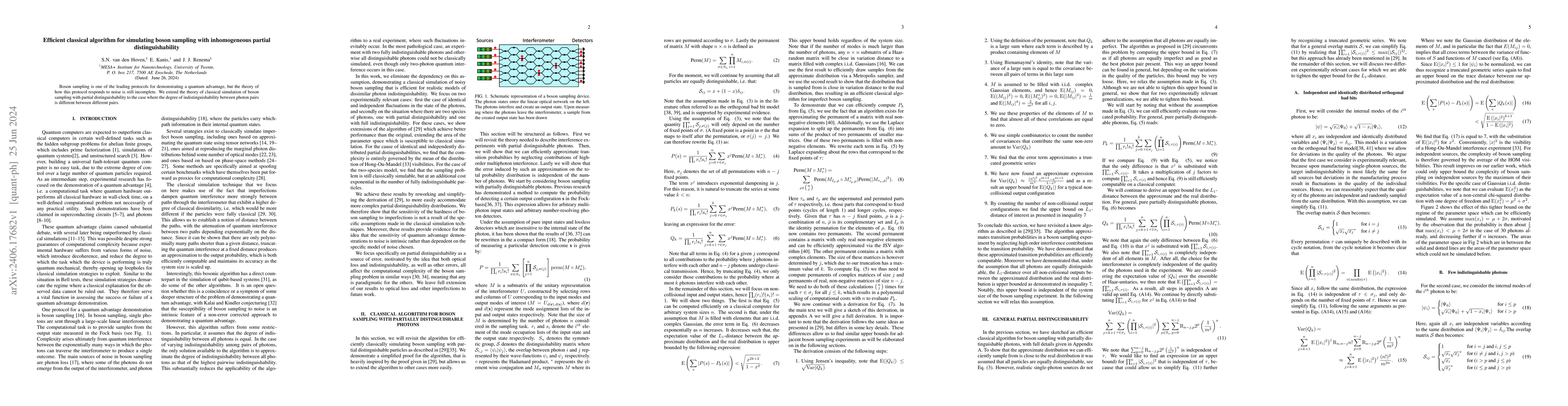
Boson sampling is one of the leading protocols for demonstrating a quantum advantage, but the theory of how this protocol responds to noise is still incomplete. We extend the theory of classical simulation of boson sampling with partial distinguishability to the case where the degree of indistinguishability between photon pairs is different between different pairs.
AI Key Findings
Get AI-generated insights about this paper's methodology, results, significance, and more — seven facets brought into focus.
Impact
Paper Details
Authors
PDF Preview
Key Terms
Citation Network
Current paper (gray), citations (green), references (blue)
Display is limited for performance on very large graphs.
Discussion 0