Evidence-invariant Sensitivity Bounds

Probabilistic networks are used to model uncertainty by combining many numerical parameters. A longstanding challenge is that sensitivity analyses—assessing how much a probability of interest changes when a parameter is varied—depend heavily on the observed evidence. In real applications, analysts must study many different evidence profiles, which makes a full, exact sensitivity analysis computationally infeasible as networks grow large. This paper tackles that gap by developing bounds on sensitivities that do not depend on the specific evidence profile, i.e., evidence-invariant bounds. The core idea is to bound the entire sensitivity function, rather than compute it exactly for every possible profile. The authors connect these bounds to the known structure of sensitivity functions, which are quotients of linear functions in the varying parameter under proportional covariation, and identify two main bound families: hyperbolic bounds and, where applicable, tighter linear bounds. They show how these bounds yield meaningful information about how much a parameter can be shifted (admissible deviation) before the most likely value of a variable of interest changes, again without needing the full network.

This approach rests on established results about sensitivity changes (notably bounds due to Chan and Darwiche) and reframes them as universal envelopes around all admissible sensitivity shapes. The bounds depend only on the original parameter value x0 and the corresponding probability p0, making them applicable across broad evidence scenarios. The paper further demonstrates that if the probability of interest relates linearly to the parameter, the bounds can be tightened, producing tighter control over both sensitivity values and admissible deviations. The practical payoff is clear: decision-makers and model builders can reason about robustness and risk without running exhaustive sensitivity analyses for every evidence pattern.

In terms of impact, these evidence-invariant bounds offer a principled, computationally cheap way to gauge robustness of probabilistic networks in real-world settings, where data are incomplete and evidence streams are numerous. They provide actionable guarantees—for example, how much a parameter can vary before the most likely outcome flips—without requiring access to or recomputation within a specific network. The bottom line for practitioners is that you can bound and reason about sensitivity and robustness using only the parameter’s original values and their associated probabilities, enabling scalable risk assessment and model validation across many possible scenarios.

Background

Probabilistic (Bayesian) networks rely on a set of numerical parameters that encode conditional probabilities. Sensitivity analysis asks how changes to a parameter x = p(b_i | π) affect a probability of interest Pr(a | e). When one parameter is varied, co-variation of other parameters in the same conditional distribution is required to preserve valid probability distributions; proportional covariation is a common and well-motivated scheme that minimizes the distance between distributions. Under proportional covariation, sensitivity functions f(x) expressing Pr(a | e) as a function of x are quotients of linear functions in x.

Sensitivity functions are thus simple in form: a ratio of two linear expressions in x, characterized by at most four constants c_j that depend on the non-varied network parameters. These properties make it feasible to compute the function with a few network propagations or by solving a small system of equations.

A key practical issue is that sensitivity results change with the evidence e. Exploring all evidence profiles in a real network quickly becomes intractable as the number of observable variables grows. This motivates the search for bounds that hold regardless of the particular evidence profile, i.e., evidence-invariant bounds.

Problem / Research Question

The central challenge is to derive and validate bounds on how a probability of interest changes when a parameter is varied, without requiring knowledge of the entire network or the current evidence profile. Specifically, the paper asks:

• Can we bound the change in a probability of interest and the parameter’s sensitivity value using only original parameter values (x0) and the corresponding probability (p0)?
• Can these bounds be made tight enough to be informative, and can they be extended to both hyperbolic and linear sensitivity functions?
• Can we translate these bounds into constraints on admissible deviations, i.e., how far a parameter can be shifted before the most likely value of a variable of interest changes, in an evidence-invariant way?

Innovation / Contribution

The paper extends prior results by showing that the well-known bounds on probability changes due to parameter shifts can be interpreted as bounds on the entire sensitivity function itself, not just on a specific x1. The main contributions are:

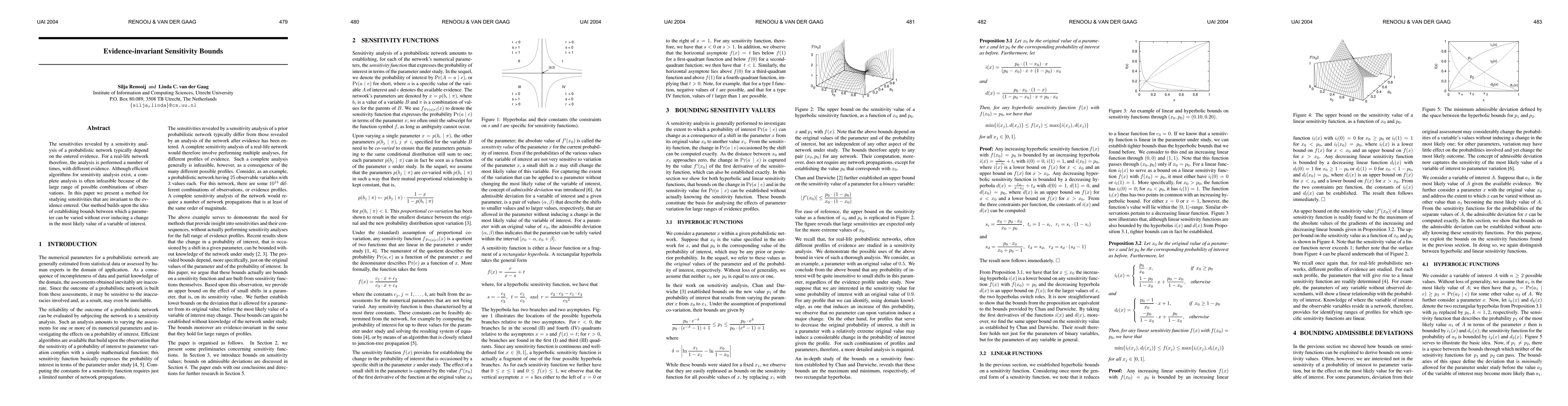
• Hyperbolic bounds: For a general (possibly non-binary) parameter, any hyperbolic sensitivity function with a given f(x0) = p0 is bounded above and below by two rectangular hyperbolas determined solely by x0 and p0 (Proposition 3.1). These bounds are independent of the network and evidence and align with Chan and Darwiche’s earlier results.
• Linear bounds: If the sensitivity function is linear in the parameter, even tighter bounds can be obtained (Proposition 3.2). This yields an explicit, tight envelope around possible linear relationships between the parameter and the probability of interest.
• Admissible deviations: The authors introduce and formalize the concept of admissible deviations, the minimal shifts in the parameter that would change the most likely value of a variable of interest. They provide explicit propositions (4.1 for hyperbolic, 4.2 for linear) that compute these minimal deviations from the intersections of the respective bounds. This gives practical, evidence-invariant guarantees about robustness of the most probable outcome under parameter variation.
• Practical implications: The bounds apply across large ranges of evidence profiles, enabling robust sensitivity reasoning without exhaustive network propagation for every profile. The results hold for non-binary variables, extend existing binary-variable results, and offer tighter control when the probability relates linearly to the parameter.

Methodology / Approach

The methodology rests on two complementary bounding strategies:

• Hyperbolic bounds (Section 3.1): For a parameter x with original value x0 and corresponding probability p0, Chan and Darwiche provide bounds on how a new probability p1 arises from varying x. The paper recasts these as bounds on the entire sensitivity function f(x) by treating the x1 replacement with x and framing the bounds as two hyperbolic envelopes i(x) and d(x) that pass through the points (0,0), (1,1), and (x0,p0) with appropriate monotonicity. These envelopes yield universal upper and lower bounds for f(x) across x in [0,1], independent of the network.
• Linear bounds (Section 3.2): When the sensitivity function is known to be linear, the paper tightens the envelope further by constructing two linear bounds il(x) and dl(x) that meet the same endpoint constraints and pass through (x0,p0). The resulting bounds provide a tight corridor for f(x) and yield an easy-to-compute upper bound on the derivative |f′(x0)|.

Admissible deviations (Section 4) use intersections of the respective upper and lower bounds for probabilities p1 and p2 (or more generally for all values of a variable A) to determine the smallest shifts (α, β) that keep the most probable value unchanged. For hyperbolic cases, Prop. 4.1 gives the minimum shifts from each bound intersection; for linear cases, Prop. 4.2 refines these to account for the intersection of linear bounds and the [0,1] value constraints.

Experiments / Evaluation

The provided text does not include empirical experiments or datasets. The work is theoretical and mathematical, with illustrative figures (Figure 1 through Figure 8) used to convey concepts such as hyperbola envelopes, linear bounds, and admissible deviations. The evaluation is therefore framed in terms of mathematical consistency with known sensitivity theory (e.g., Chan and Darwiche), and in-context demonstrations (via described examples and figures) that the bounds behave intuitively across different original parameter values and probability configurations. Future work would likely involve empirical validation on real-world networks to quantify bound tightness and practical savings in sensitivity workflows.

Key Results

• Hyperbolic bounds: For any hyperbolic sensitivity function f(x) with f(x0)=p0, there exist two hyperbolic bounds i(x) and d(x) that bound f(x) from below and above on [0,1], computed from the triple (x0, p0) and the asymptotic constraints. These bounds are equivalent to Chan and Darwiche’s results and apply to general, non-binary parameters.
• Sensitivity bound: The derivative bound |f′(x0)| for hyperbolic cases matches the known upper bound derived by Chan and Darwiche for binary variables, and the paper shows this extends to general variables.
• Linear bounds: If the sensitivity function is linear, il(x) and dl(x) yield tighter bounds than the hyperbolic envelopes. The maximum possible |f′(x0)| is bounded by the maximum gradient of these linear bounds, and the entire envelope lies below the hyperbolic bound surfaces.
• Admissible deviation: Propositions 4.1 and 4.2 provide explicit formulas to compute the minimum admissible deviations (α, β) for hyperbolic and linear cases, respectively, based on intersections of the corresponding bounds. This yields concrete margins within which parameter variation cannot flip the most likely value of the variable of interest.
• Evidence-invariance: The core insight is that these bounds hold across large ranges of evidence profiles, enabling robustness analysis without enumerating all evidence configurations.

Practical Applications

The results offer researchers and practitioners a scalable toolkit for robustness assessment in probabilistic networks.

• Model validation: Before deploying a model, assess whether plausible parameter variations could change key decisions by checking admissible deviations derived from x0 and p0.
• Risk assessment under uncertainty: When data are scarce, these bounds provide guaranteed confinement on how much a parameter can drift without altering the most likely outcomes, aiding conservative decision-making.
• Tool integration: The approach can be embedded into sensitivity-analysis software to provide fast, evidence-invariant guards, reducing the need for repeated full-network propagations across many evidence profiles.
• Diagnostic prioritization: By identifying parameters with small admissible deviations, practitioners can prioritize data collection or expert elicitation to reduce critical uncertainty.

Limitations & Considerations

While powerful, the framework rests on several assumptions and has boundaries:

• Proportional covariation: The derivations assume proportional co-variation when varying a parameter. Deviations from this co-variation scheme could affect the bounds’ validity.
• Non-extreme probabilities: The analysis excludes x0 and p0 equal to 0 or 1. Near-extreme values may require careful handling or alternative bounding forms.
• General vs. linear cases: Tight bounds hinge on whether the sensitivity function is truly linear. In practice, one must diagnose or test which functional form applies in a given network scenario.
• Higher-dimensional sensitivity: The bounds address single-parameter perturbations. Extending to simultaneous multi-parameter changes, or exploring interactions across many parameters, remains open.
• Network structure effects: While the bounds are evidence-invariant, their usefulness in very large networks with complex dependencies should be empirically assessed to understand practical tightness and computational benefits.
• Extensions to continuous or multi-valued variables: The text generalizes beyond binary variables, but deeper treatment or empirical validation for multi-valued or continuous nodes would be valuable.
• Runtime integration: Real-world applicability depends on implementing efficient routines to detect whether a given sensitivity is hyperbolic or linear and to compute intersections for admissible deviations automatically.

Probabilistic networks are powerful, but their answers can depend heavily on what evidence you’ve observed. In real life, you’d like to know whether small changes in a parameter (say, a probability in a conditional distribution) might flip a decision, regardless of the exact network details. This paper shows how you can bound such effects without re-running sensitivity analyses for every possible piece of evidence. The key idea is that the sensitivity of a probability of interest to a parameter can be described by a simple mathematical shape: either a straight line or a fragment of a hyperbola. Crucially, you can bound how much the probability and its sensitivity can change using only the parameter’s original value and the original probability of interest, x0 and p0, without knowing the full network structure. These bounds come in two flavors: hyperbolic bounds that apply generally, and tighter linear bounds when the relationship is known to be linear. By combining these bounds, the authors derive both how much a parameter can move (the admissible deviation) before the most likely outcome changes, and how large the sensitivity can be. Importantly, these results hold across wide ranges of evidence profiles, which means one bound can be useful for many potential observations, reducing the need for exhaustive re-analysis. The practical upshot is a toolkit for robustness analysis that scales to large networks: you can reason about parameter changes and their consequences without committing to a full sensitivity study for every possible observation scenario. This sets the stage for future work that extends these “evidence-invariant” bounds to higher-order sensitivities and to more complex, real-world systems.

Imagine you have a big recipe book that predicts how tasty a dish will be, based on dozens of small ingredients. You’re worried that changing one ingredient a little might suddenly make the dish taste worse, but you don’t want to re-test every possible kitchen situation to know for sure. This paper gives you a shortcut: it shows you safe margins for each ingredient that tell you, no matter which exact tasting notes you’re dealing with (the “evidence”), how much you can tweak that ingredient before the final dish’s top flavor changes to something else. It’s like knowing: if you started with this amount of salt and this level of sweetness, you can tweak each by a certain amount and your dish’s best choice of flavor stays the same. They do this with two kinds of math shapes—hyperbolas and straight lines—to describe how ingredient tweaks roll into taste changes. When the relationship is simply linear, the bounds get even tighter.

They also introduce a handy concept called admissible deviation. Think of it as a safety margin: the smallest amount you’d have to change an ingredient before the dish’s most likely winner flavor changes. This helps cooks and model builders decide which ingredients deserve careful measurement and which changes can be ignored. The big idea is that you don’t need to cook every possible kitchen scenario to know how robust your predictions are—you can rely on these universal bounds that depend only on the starting value of the ingredient and the baseline probability of a flavor outcome. That makes testing big, tricky recipes of uncertainty much more practical and reliable.

So, what did they discover? They showed that you can bound how much a parameter can influence a probability of interest without knowing the whole network or every piece of evidence. If the relationship is more like a straight line, you can bound both the sensitivity and the safe variation more tightly. And you get concrete margins (admissible deviations) that tell you exactly when the most likely outcome could flip. This is a win for anyone building or using probabilistic models in the real world, because it makes robustness checks faster, clearer, and less brittle to the unknowns you can’t control.

Admissible deviation: Bounds on how far a parameter x can be shifted before the most likely value of the variable of interest changes — "An admissible deviation for a variable of interest and a given parameter, is a pair of values ( α, β ) that describe the shifts to smaller values and to larger values, respectively, that are allowed in the parameter without inducing a change in the most likely value of the variable of interest."

• Empirical validation across diverse real-world networks: quantify how often hyperbolic versus linear bounds tightly bound actual sensitivity functions and the practical savings in propagation runs.
• Multi-parameter sensitivity: extend the evidence-invariant bounds to simultaneous variation of multiple parameters, including potential interactions and covariances beyond proportional covariation.
• Generalization to high-cardinality or continuous variables: provide explicit bounding forms and propositions for variables with more than two values or continuous domains, and validate their tightness.
• Robustness to covariation deviations: assess how sensitive the bounds are if the assumed proportional covariation is violated or only approximately held in practice.
• Dynamic or temporal networks: explore how these bounds translate to dynamic Bayesian networks where evidence unfolds over time and parameters may evolve.
• Integration with learning workflows: develop practical guidelines and software support to automatically detect when a sensitivity function is hyperbolic versus linear in real networks and compute admissible deviations accordingly.
• Boundary behavior near x0 or p0 close to 0 or 1: provide specialized treatments or alternative bounds for extreme parameter regimes that were excluded in the analysis.
• Empirical impact on decision-making: study how using these bounds changes risk assessment, model validation, and decision confidence in applied domains (medicine, engineering, finance, etc.).

Immediate Applications

• Healthcare: Use evidence-invariant bounds to assess robustness of diagnostic Bayesian networks to parameter uncertainty across diverse patient evidence, avoiding full sensitivity analyses for every patient; relies on discrete Bayesian networks, proportional covariation, and the ability to compute p0 from the current x0.
• Finance: Bound the impact of parameter estimation error on probabilities driving credit-risk decisions in Bayesian risk models across multiple market scenarios; no full re-propagation for each scenario required; assumes the proportional covariation rule and access to x0 and p0.
• Robotics and autonomous systems: Guarantee safe decision-making under sensor noise by bounding how parameter uncertainty affects action-selection probabilities across varying sensory inputs; requires a probabilistic model of perception and discrete states.
• Industrial monitoring and fault diagnosis: Bound the effect of sensor calibration drift on the probability of fault states across many sensor profiles; enables robustness checks without exhaustive re-analysis.
• Knowledge-based diagnostic systems in engineering or medicine: Rapidly assess robustness across evidence profiles without running complete sensitivity analyses for every profile; depends on having x0 and p0 for the probability of interest.

Long-Term Applications

• Automated robustness tooling for large-scale Bayesian networks used in healthcare, finance, and manufacturing: compute evidence-invariant and admissible-deviation bounds for many variables; requires scalable inference and clear visualization; may depend on attaching to existing model repository.
• Extension to higher-order sensitivities and multi-parameter interactions: to bound effects beyond a single parameter; requires new theory and algorithms.
• Real-time or streaming-data decision support: Bound potential changes quickly as evidence updates; requires near-real-time inference and incremental updating.
• Regulatory and auditing frameworks: Use evidence-invariant bounds as a robustness metric; requires standardization and validation across domains.