Publication
Metrics
AI Quick Summary
This paper introduces a penalized least-squares method ensuring fitted value invariance under linear transformations, essential for categorical predictors and interactions. The proposed method achieves comparable computational efficiency to ridge regression while offering this invariance, and it provides optimal tuning parameter estimators with studied asymptotic properties.
Paper Preview
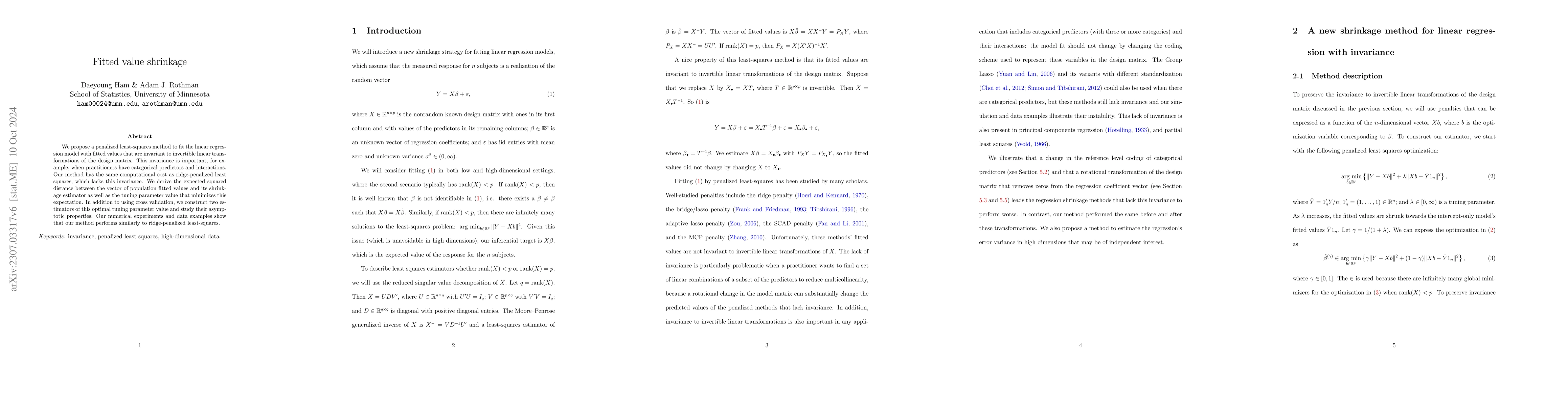
Abstract
We propose a penalized least-squares method to fit the linear regression model with fitted values that are invariant to invertible linear transformations of the design matrix. This invariance is important, for example, when practitioners have categorical predictors and interactions. Our method has the same computational cost as ridge-penalized least squares, which lacks this invariance. We derive the expected squared distance between the vector of population fitted values and its shrinkage estimator as well as the tuning parameter value that minimizes this expectation. In addition to using cross validation, we construct two estimators of this optimal tuning parameter value and study their asymptotic properties. Our numerical experiments and data examples show that our method performs similarly to ridge-penalized least-squares.
AI Key Findings
Get AI-generated insights about this paper's methodology, results, significance, and more — seven facets brought into focus.
Impact
Paper Details
Authors
PDF Preview
Key Terms
Citation Network
Current paper (gray), citations (green), references (blue)
Display is limited for performance on very large graphs.
Discussion 0