Background
The paper sits at the intersection of causal graphical models and linear structural equation modeling. It treats variables as nodes in a directed acyclic graph (DAG) with arrows representing direct causal effects and bidirected edges representing correlations induced by unobserved common causes. All interactions are assumed linear. A central concern is the Identification Problem: given a fixed graph and observed covariances among the observed variables, can one uniquely recover the direct causal effects (the edge coefficients) that generated the data? The authors build on foundational ideas like Instrumental Variables (IV) and Wright’s method of path coefficients, but extend them to models where conditional independences are sparse or where errors are correlated.
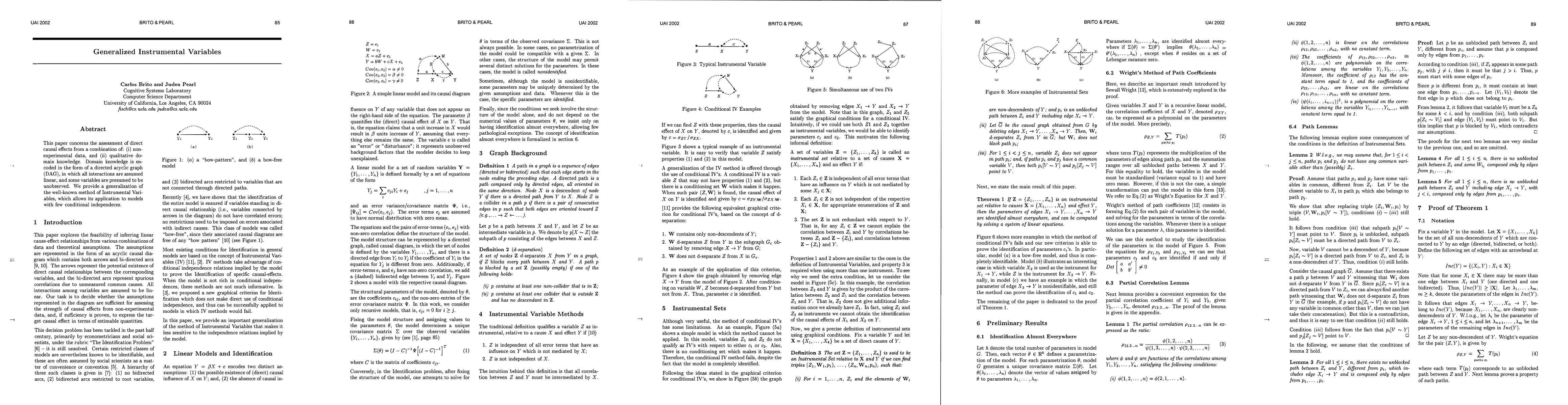
A key restriction discussed is the bow-free class, where the graph contains no bow patterns—instances where a direct causal edge and a correlated error connect the same two variables. Earlier work showed identifiability in bow-free models, but real-world graphs often violate this or offer few independences to exploit. The authors aim to relax reliance on independence by introducing a new criterion that uses multiple instruments collectively rather than relying on a single instrument that satisfies classical IV conditions.
Problem / Research Question
The core question asks when and how one can identify the direct causal effects of a set of causes X on a target Y using non-experimental data in linear models with possible unobserved confounding. When traditional IV methods cannot be applied due to a paucity of conditional independences, is there a graphical construction that still yields identification? The paper seeks a general condition under which the edge coefficients X1 → Y, ..., Xn → Y are identifiable almost everywhere and a practical method to compute them.
Innovation / Contribution
The principal contribution is the formal definition of an Instrumental Set (Definition 3) relative to a set of causes X and a target Y. An instrumental set is a collection of variables Z1, ..., Zn, together with conditioning sets W1, ..., Wn and unblocked paths p1, ..., pn, that satisfy three graphical conditions: (i) each Zi and Wi are non-descendants of Y and Zi lies on an unblocked path to Y that includes the edge Xi → Y; (ii) after deleting all direct Y-connecting edges from the graph, Wi d-separates Zi from Y; and (iii) no Zj reappears on the same unblocked path with a conflicting direction, ensuring non-redundancy.
Theorem 1 then shows that if such an instrumental set exists for a given X and Y, the parameters of the edges Xi → Y are identified almost everywhere and can be computed by solving a linear system. A central methodological device is Wright’s path-coefficient framework, which expresses correlations as polynomials in the edge parameters via unblocked paths. The authors exploit a matrix Q—the coefficient matrix of the linear system—whose determinant is a non-trivial polynomial in the model parameters. Since the zero-set of a non-zero polynomial has Lebesgue measure zero, det(Q) ≠ 0 almost everywhere, ensuring identifiability in almost all parameterizations.
The approach also shows how to estimate the system from data: the entries of Q are computable from correlations among observed variables, and the right-hand sides of the linear equations are expressible in terms of observed covariances. Importantly, the method permits using multiple instruments jointly, mitigating situations where single IVs or simple conditioning fail.
Methodology / Approach
The analysis begins by fixing a target Y and the candidate direct causes X = {X1, ..., Xn}. Each edge Xi → Y has an associated parameter Ai. The authors consider the set Inc(Y) of all edges into Y and partition the parameters accordingly. For each Zi, they couple a conditioning set Wi and a path Pi that unblockedly connects Zi to Y via the edge Xi → Y. They then derive Wright’s equations for the pair (Zi, Y) and manipulate these equations to express the observed correlations as linear combinations of the edge parameters, with known coefficients dependent on the observed covariances and the graph structure.
Crucially, Lemmas 2–5 establish structural constraints that prevent unwanted overlap among the Pi and the Wi, ensuring that the resulting linear system has a chance to identify the Xi → Y parameters. Lemma 6 shows that any unblocked path from a non-descendant Z to Y must cross exactly one edge in Inc(Y), which is essential to linearize the system. Building on these, the authors formulate a system of equations (Eq. 6 and subsequent expressions) whose unknowns are A1, ..., An. They prove that the coefficient matrix Q has a determinant that is a non-trivial polynomial in the model’s parameters (Lemma 8), guaranteeing identifiability almost everywhere.
For estimation, they show that each entry of Q is computable from data (the correlations among Z, W, and Y), and that the right-hand sides of the equations are also expressible in terms of observable correlations. Therefore, the parameters A1, ..., An can be solved from data by inverting Q (where det(Q) ≠ 0) and obtaining a unique solution for the edge coefficients.
Experiments / Evaluation
The paper presents a theoretical development with formal proofs rather than empirical experiments. The Evaluation is mathematical: it proves Lemma 2–8 and Theorem 1, establishes the identifiability almost everywhere, and sketches how the coefficients can be estimated from sample covariances. The Appendix contains the proofs of the technical lemmas, including the construction of Wright’s equations in this broadened setting and the polynomial nature of the determinant argument.
Key Results
The central result is Theorem 1: if Z = {Z1, ..., Zn} forms an Instrumental Set relative to X = {X1, ..., Xn} and Y, then the parameters of the edges Xi → Y are identified almost everywhere and can be computed by solving a system of linear equations. Supporting results include Lemmas 2–6, which establish the path-structural properties that guarantee the linearization, Lemma 7, which shows that the coefficients reduce to a linear function of a finite set of edge-parameters, and Lemma 8, which proves that the determinant of the system’s coefficient matrix is a non-trivial polynomial, ensuring identifiability almost everywhere. The paper also emphasizes that a single graph can admit different instrumental-set constructions, enabling identification in models where traditional IV methods would fail.
Practical Applications
The instrumental-set framework broadens the practical toolkit for causal inference in fields where observational data are all that is available and where latent confounding cannot be ignored. It is particularly relevant to econometrics, social sciences, and any domain that relies on linear, recursive models with potential correlations among error terms. The method enables the identification of multiple direct effects from a single Y, using several instruments in tandem, provided the graphical criteria can be satisfied. This can be especially valuable in complex systems where the independence structure is sparse and where bow patterns would otherwise block identification.
Limitations & Considerations
A fundamental limitation is that identifiability is guaranteed only almost everywhere; there exist measure-zero parameter configurations where det(Q) = 0 and identification fails. The approach also relies on a correct specification of the causal graph, linearity of all interactions, and the assumption that the error terms can be correlated in a controlled way (as encoded by the bidirected edges). In practice, estimating the system requires accurate estimation of covariances from finite samples, which may be sensitive to sampling noise, model misspecification, and measurement error. Finally, while the method extends IV applicability, it does not automatically solve all identification challenges: researchers must still verify the instrument-set conditions for their particular graph and data, and recognize that some models may remain non-identifiable under these criteria.
Discussion 0