Space-time fractional equations and the related stable processes at random time

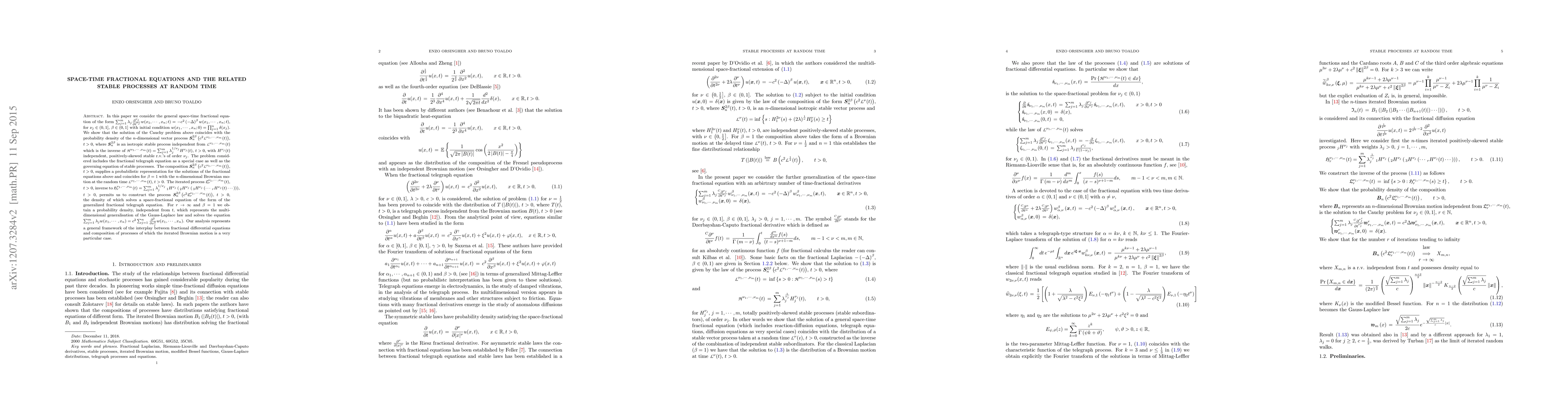
In this paper we consider the general fractional equation \sum_{j=1}^m \lambda_j \frac{\partial^{\nu_j}}{\partial t^{\nu_j}} w(x_1,..., x_n ; t) = -c^2 (-\Delta)^\beta w(x_1,..., x_n ; t), for \nu_j \in (0,1], \beta \in (0,1] with initial condition w(x_1,..., x_n ; 0)= \prod_{j=1}^n \delta (x_j). The solution of the Cauchy problem above coincides with the distribution of the n-dimensional process \bm{S}_n^{2\beta} \mathcal{L} c^2 {L}^{\nu_1,..., \nu_m} (t) \r, t>0, where \bm{S}_n^{2\beta} is an isotropic stable process independent from {L}^{\nu_1,..., \nu_m}(t) which is the inverse of {H}^{\nu_1,..., \nu_m} (t) = \sum_{j=1}^m \lambda_j^{1/\nu_j} H^{\nu_j} (t), t>0, with H^{\nu_j}(t) independent, positively-skewed stable r.v.'s of order \nu_j. The problem considered includes the fractional telegraph equation as a special case as well as the governing equation of stable processes. The composition \bm{S}_n^{2\beta} (c^2 {L}^{\nu_1,..., \nu_m} (t)), t>0, supplies a probabilistic representation for the solutions of the fractional equations above and coincides for \beta = 1 with the n-dimensional Brownian motion at the time {L}^{\nu_1,..., \nu_m} (t), t>0. The iterated process {L}^{\nu_1,..., \nu_m}_r (t), t>0, inverse to {H}^{\nu_1,..., \nu_m}_r (t) =\sum_{j=1}^m \lambda_j^{1/\nu_j} _1H^{\nu_j} (_{2}H^{\nu_j} (_3H^{\nu_j} (... _{r}H^{\nu_j} (t)...))), t>0, permits us to construct the process \bm{S}_n^{2\beta} (c^2 {L}^{\nu_1,..., \nu_m}_r (t)), t>0, the distribution of which solves a space-fractional generalized telegraph equation. For r \to \infty and \beta = 1 we obtain a distribution which represents the n-dimensional generalisation of the Gauss-Laplace law and solves the equation \sum_{j=1}^m \lambda_j w(x_1,..., x_n) = c^2 \sum_{j=1}^n \frac{\partial^2}{\partial x_j^2} w(x_1,..., x_n).