Thin film optics computations in a high-level programming language environment: tutorial

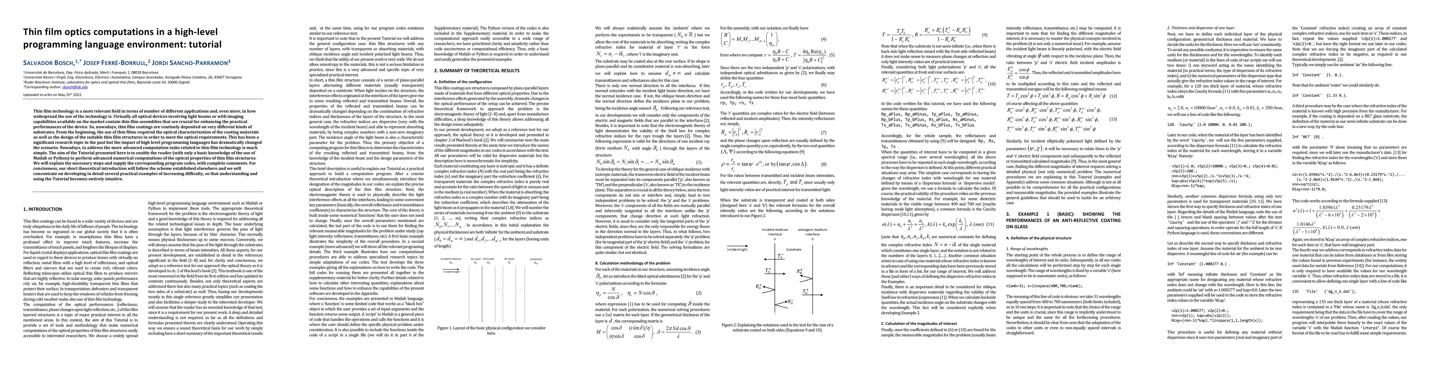
Thin film technology is a most relevant field in terms of number of different applications and, even more, in how widespread the use of the technology is. Virtually all optical devices involving light beams or with imaging capabilities available on the market contain thin film assemblies that are crucial for enhancing the practical performances of the device. So, nowadays, thin film coatings are routinely deposited on very different kinds of substrates. From the beginning, the use of thin films required the optical characterization of the coating materials as well as the design of the suitable thin film structures in order to meet the optical requirements. This has been a significant research topic in the past but the impact of high level programming languages has dramatically changed the scenario. Nowadays, to address the more advanced computation tasks related to thin film technology is much simple. The aim of the Tutorial presented here is to enable the reader (with only a basic knowledge of the use of Matlab or Python) to perform advanced numerical computations of the optical properties of thin film structures. We will explain the necessary steps and supply the corresponding program codes, with complete comments. For conciseness, our short theoretical introduction will follow the scheme established elsewhere and we will concentrate on developing in detail several practical examples of increasing difficulty, so that understanding and using the Tutorial becomes entirely intuitive.