Contents
1211.4552
A Dataset for StarCraft AI & an Example of Armies Clustering
Gabriel Synnaeve and Pierre Bessi` ere
Coll` ege de France, CNRS, Grenoble University, LIG [email protected] [email protected] and
Abstract
This paper advocates the exploration of the full state of recorded real-time strategy (RTS) games, by human or robotic players, to discover how to reason about tactics and strategy. We present a dataset of StarCraft 1 games encompassing the most of the games' state (not only player's orders). We explain one of the possible usages of this dataset by clustering armies on their compositions. This reduction of armies compositions to mixtures of Gaussian allow for strategic reasoning at the level of the components. We evaluated this clustering method by predicting the outcomes of battles based on armies compositions' mixtures components.
Introduction
Real-time strategy (RTS) games AI is not yet at a level high enough to compete with trained/skilled human players. Particularly, adaptation to different strategies (of which army composition) and to tactics (army moves) are strong indicators of human-played games (Hagelb¨ ack and Johansson 2010). So, while micro-management (low level units control) has known tremendous improvements in recent years, the broadest high-level strategic reasoning is not yet an exemplary feature neither of commercial games nor of StarCraft AI competitions' entries. At best, StarCraft bots have an estimation of the available technology of their opponents and use rules encoding players' knowledge to adapt their strategy. We believe that better strategic reasoning is a matter of abstracting and combining the low level states at an expressive higher level of reasoning. Our approach will be to learn unsupervised representations of low-level features.
We worked on StarCraft: Brood War, which is a canonical RTS game, as Chess is to board games. It had been around since 1998, has sold 10 millions licenses and was the best competitive RTS for more than a decade. There are 3 factions (Protoss, Terran and Zerg) that are totally different in terms of units, build trees / tech trees (directed acyclic graphs of the buildings and technologies) and thus gameplay styles. StarCraft and most RTS games provide a tool to record game logs into replays that can be re-simulated by
Copyright c © 2024, Association for the Advancement of Artificial Intelligence (www.aaai.org). All rights reserved.
1 StarCraft and its expansion StarCraft: Brood War are trademarks of Blizzard Entertainment TM
the game engine. That is this trace mechanism that we used to download and simulate games of professional gamers and highly skilled international competitors.
This paper is separated in two parts. The first part explains what is in the dataset of StarCraft games that we put together. The second part showcases army composition reduction to a mixture of Gaussian distributions, and give some evaluation of this clustering.
Related Work
There are several ways to produce strategic abstractions: from using high-level gamers' vocabulary, and the game rules (build/tech trees), to salient low-level (shallow) features. Other ways include combining low-level and higherlevel strategic representation and/or interdependencies between states and sequences.
Case-based reasoning (CBR) approaches often use extensions of build trees as state lattices (and sets of tactics for each state) as for (Aha, Molineaux, and Ponsen 2005; Ponsen and Spronck 2004) in Wargus. Onta˜ n´ on et al. (2007) base their real-time case-based planning (CBP) system on a plan dependency graph which is learned from human demonstration in Wargus. In (Mishra, Onta˜ n´ on, and Ram 2008), they use 'situation assessment for plan retrieval' from annotated replays, which recognizes distance to behaviors (a goal and a plan), and selected only the low-level features with the higher information gain. Hsieh and Sun (2008) based their work on (Aha, Molineaux, and Ponsen 2005) and used StarCraft replays to construct states and building sequences. Strategies are choices of building construction order in their model.
Schadd, Bakkes, and Spronck (2007) describe opponent modeling through hierarchically structured models of the opponent behavior and they applied their work to the Spring RTS game (Total Annihilation open source clone). Balla and Fern (2009) applied upper confidence bounds on trees (UCT: a Monte-Carlo planning algorithm) to tactical assault planning in Wargus, their tactical abstraction combines units hit points and locations. In (Synnaeve and Bessi` ere 2011b), they predict the build trees of the opponent a few buildings before they are built. Another approach is to use the gamers' vocabulary of strategies (and openings) to abstract even more what strategies represent (a set of states, of sequences and of intentions) as in (Weber and Mateas 2009;
Synnaeve and Bessi` ere 2011a). Dereszynski et al. (2011) used an hidden Markov model (HMM) whose states are extracted from (unsupervised) maximum likelihood on a StarCraft dataset. The HMM parameters are learned from unit counts (both buildings and military units) every 30 seconds and 'strategies' are the most frequent sequences of the HMMstates according to observations.
Few models have incorporated army compositions in their strategy abstractions, except sparsely as an aggregate or boolean existence of unit types. Most strategy abstractions are based on build trees (or tech trees), although a given set of buildings can produce different armies. What we will present here is complementary to these strategic abstractions and should help the military situation assessment.
Dataset
We downloaded more than 8000 replays to keep 7649 uncorrupted, 1 vs. 1 replays from professional gamers leagues and international tournaments of StarCraft, from specialized websites 234 . We then ran them using Brood War API 5 and dumped: units' positions, regions' positions, pathfinding distance between regions, resources (every 25 frames), all players' orders, vision events (when units are seen) and attacks (types, positions, outcomes). Basically, we recorded every BWAPI event, plus interesting states and attacks. The dataset is freely available 6 , the source code and a documentation are also provided 7
Regions
Forbus, Mahoney, and Dill (2002) have shown the importance of qualitative spatial reasoning, and it would be too space-consuming to dump the ground distance of every position to any other position. For these reasons, we discretized StarCraft maps in two types of regions:
- Brood War Terrain Analyzer 8 produced regions from a pruned Voronoi diagram on walkable terrain (Perkins 2010). Chokes are the boundaries of such regions.
- As battles often happens at chokes, we also produced choke-dependent regions (CDR), which are created by doing an additional (distance limited) Voronoi tessellation spawned at chokes. This regions set is
CDR = ( regions \ chokes ) ∪ chokesAttacks
We trigger an attack tracking heuristic when one unit dies and there are at least two military units around. We then update this attack until it ends, recording every unit which took part in the fight. We log the position, participating units and
2 http://www.teamliquid.net 3 http://www.gosugamers.net 4 http://www.iccup.com 5 BWAPI http://code.google.com/p/bwapi/ 6 http://emotion.inrialpes.fr/people/ synnaeve/TLGGICCUP_gosu_data.7z 7 http://snippyhollow.github.com/bwrepdump/ 8 BWTA http://code.google.com/p/bwta/fallen units for each player, the attack type and of course the attacker and the defender. Algorithm 1 shows how we detect attacks.
We annotated attacks by four types (but researchers can also produce their own annotations given the state available):
- ground attacks, which may use all types of units (and so form the large majority of attacks).
- air raids, air attacks, which can use only flying units.
- invisible (ground) attacks, which can use only a few specific units in each race (Protoss Dark Templars, Terran Ghosts, Zerg Lurkers).
- drop attacks, which need a transport unit (Protoss Shuttle, Terran Dropship, Zerg Overlord with upgrade).
Algorithm 1 Simplified attack tracking heuristic for extraction from games. The heuristics to determine the attack type and the attack radius and position are not described here. They look at the proportions of units types, which units are firing and the last actions of the players.
glyph[negationslash]
list tracked attacks function UNIT DEATH EVENT( unit ) tmp ← tracked attacks.which contains ( unit ) if tmp = ∅ then tmp.update ( unit ) glyph[triangleright] ⇔ update ( tmp, unit ) else tracked attacks.push ( attack ( unit )) end if end function function ATTACK( unit ) glyph[triangleright] new attack constructor glyph[triangleright] self ⇔ this self.convex hull ← default hull ( unit ) self.type ← attack type ( update ( self, unit )) return self end function function UPDATE( attack, unit ) attack.update hull ( unit ) glyph[triangleright] takes units ranges into account c ← get context ( attack.convex hull ) self.units involved.update ( c ) self.tick ← default timeout () return c end function function TICK UPDATE self.tick ← self.tick -1 if self.tick < 0 then self.destruct () end if end functionInformation in the dataset
Table 1 shows some metrics about the dataset. Note that the numbers of attacks for a given race have to be divided by (approximatively) two in a given non-mirror match-up. So, there are 7072 Protoss attacks in PvP and there are not 70,089 attacks by Protoss in PvT but about half that.
| match-up | PvP | PvT | PvZ | TvT | TvZ | ZvZ |
|---|---|---|---|---|---|---|
| number of games | 445 | 2408 | 2027 | 461 | 2107 | 199 |
| number of attacks | 7072 | 70089 | 40121 | 16446 | 42175 | 2162 |
| mean attacks/game | 15.89 | 29.11 | 19.79 | 35.67 | 20.02 | 10.86 |
| mean time (frames) / game | 32342 | 37772 | 39137 | 37717 | 35740 | 23898 |
| mean time (minutes) / game | 22.46 | 26.23 | 27.18 | 26.19 | 24.82 | 16.60 |
| actions issued (game engine) / game | 24584 | 33209 | 31344 | 26998 | 29869 | 21868 |
| mean regions / game | 19.59 | 19.88 | 19.69 | 19.83 | 20.21 | 19.31 |
| mean CDR / game | 41.58 | 41.61 | 41.57 | 41.44 | 42.10 | 40.70 |
| mean ground distance 9 region ↔ region | 2569 | 2608 | 2607 | 2629 | 2604 | 2596 |
| mean ground distance 10 CDR ↔ CDR | 2397 | 2405 | 2411 | 2443 | 2396 | 2401 |
By running the recorded games (replay) through StarCraft, we were able to recreate the full state of the game. Time is always expressed in game frames (24 frames per second). We recorded three types of files:
- general data ( *.rgd files): records the players' names, the map's name, and all information about events like creation (along with morph ), destruction , discovery (for one player), change of ownership (special spell/ability), for each units. It also shows attack events (detected by a heuristic, see below) and dumps the current economical situation every 25 frames: mineral, gas, supply (count and total: maxsupply).
- order data ( *.rod files): records all the orders which are given to the units (individually) like move , harvest , attack unit , the orders positions and their issue time.
- location data ( *.rld files): records positions of mobile units every 100 frames, and their position in regions and choke-dependent regions if they changed since last measurement. It also stores ground distances (pathfindingwise) matrices between regions and choke-dependent regions in the header.
From this data, one can recreate most of the state of the game: the map key characteristics (or load the map separately), the economy of all players, their tech (all researches and upgrades), all the buildings and units, along with their orders and their positions.
Armies composition
We will consider units engaged in these attacks as armies and will seek a compact description of armies compositions.
Armies clustering
The idea behind armies clustering is to give one 'composition' label for each army depending on its composing ratio of the different unit types. Giving a 'hard' (unique) label for each army does not work well because armies contain different components of unit types combinations. For instance, a Protoss army can have only a 'Zealots+Dragoons' component, but it will often just be one of the components (sometimes the backbone) of the army composition, augmented for instance with 'High Templars+Archons'.
Because a hard clustering is not an optimal solution, we used a Gaussian mixture model (GMM), which assumes that an army is a mixture (i.e. weighted sum) of several (Gaussian) components. We present the model in the Bayesian programming framework (Diard, Bessi` ere, and Mazer 2003): we first describe the variables, the decomposition (independence assumptions) and the forms of the distribution. Then, we explain how we identified (learned) the parameters and lay out the question that we will ask this model in the following parts.
Variables
- C ∈ J c 1 . . . c K K , our army clusters/components ( C ). There are K units clusters and K depends on the race (the mixture components are not the same for Protoss/Terran/Zerg).
glyph[negationslash]
- U ∈ ([0 , 1] . . . [0 , 1]) (length N ), our N dimensional unit types ( U ) proportions, i.e. U ∈ [0 , 1] N . N is dependent on the race and is the total number of unit types. For instance, an army with equal numbers of Zealots and Dragoons (and nothing else) is represented as { U Zealot = 0 . 5 , U Dragoon = 0 . 5 , ∀ ut = Zealot | Dragoon U ut = 0 . 0 } , i.e. U = (0 . 5 , 0 . 5 , 0 , . . . , 0) if Zealots and Dragoons are the first two components of the U vector. So ∑ i U i = 1 whatever the composition of the army.
Decomposition: For the M battles, the armies compositions are independent across battles, and the unit types proportions vector (army composition) is generated by a mixture of Gaussian components and thus U i depends on C i .
Forms
- P( U i | C i ) mixture of Gaussian distributions:
- P( C ) = Categorical ( K,p )
Identification (learning): We learned the Gaussian mixture models (GMM) parameters with the expectationmaximization (EM) algorithm on 5 to 15 mixtures with spherical, tied, diagonal and full co-variance matrices, using scikit-learn (Pedregosa et al. 2011). We kept the best scoring models (by varying the number of mixtures) according to the Bayesian information criterion (BIC) (Schwarz 1978).
Let θ = ( µ 1: K , σ 2 1: K ) , being respectively the K different N -dimensional means ( µ 1: K ) and the variances ( σ 2 1: K ) of the normal distributions. Initialize θ randomly, and let
Iterate until convergence (of θ ):
Question: For the i th battle (one army with units u ):
Counter compositions
In a battle, there are two armies (one for each players), we can thus apply this clustering to both the armies. If we have K clusters and N unit types, the opponent has K ′ clusters and N ′ unit types. We introduce EU and EC , respectively with the same semantics as U and C but for the enemy. In a given battle, we observe u and eu , respectively our army composition and the enemy's army composition. We can ask P( C | U = u ) and P( EC | EU = eu ) .
As StarCraft unit types have strengths and weaknesses against other types, we can learn which clusters should beat other clusters (at equivalent investment) as a probability table. We use Laplace's law of succession ('add-one smoothing') by counting and weighting according to battles results ( c > ec means ' c beats ec ', i.e. we won against the enemy):
Results
We used the dataset presented in this paper to learn all the parameters and perform the benchmarks (by setting 100 test matches aside and learning on the remaining of the dataset). First, we analyze the posteriors of clustering only one army and then we evaluated the clustering as a mean to predict outcomes of battles.
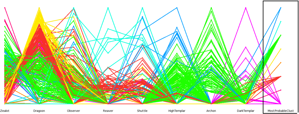
Posterior analysis: Figure 1 shows a parallel plot of army compositions . We removed the less frequent unit types to keep only the 8 most important unit types of the PvP matchup, and we display a 8 dimensional representation of the army composition, each vertical axis represents one dimension. Each line (trajectory in this 8 dimensional space) represents an army composition (engaged in a battle) and gives the percentage of each of the unit types. These lines (armies) are colored with their most probable mixture component, which are shown in the rightmost axis. We have 8 clusters (Gaussian mixtures components): this is not related to the 8 unit types used as the number of mixtures was chosen by BIC score. Expert StarCraft players will directly recognize the clusters of typical armies, here are some of them:
- Light blue corresponds to the 'Reaver Drop' tactical squads, which aims are to transport (with the flying Shuttle) the slow Reaver (zone damage artillery) inside the opponent's base to cause massive economical damages.
- Red corresponds to the 'Nony' typical army that is played in PvP (lots of Dragoons, supported by Reaver and Shuttle).
- Green corresponds to a High Templar and Archon-heavy army: the gas invested in such high tech units makes it that there are less Dragoons, completed by more Zealots (which cost no gas).
- Purple corresponds to Dark Templar ('sneaky', as Dark Templars are invisible) special tactics (and opening).
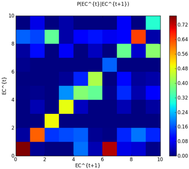
Figure 2 showcases the dynamics of clusters components: P( EC t | EC t +1 , for Zerg (vs Protoss) for ∆ t of 2 minutes. The diagonal components correspond to those which do not change between t and t +1 ( ⇔ t +2 minutes), and so it is normal that they are very high. The other components show the shift between clusters. For instance, the first line seventh column (in (0,6)) square shows a brutal transition from the first component (0) to the seventh (6). This may be the production of Mutalisks 11 from a previously very low-tech army (Zerglings).
A soft rock-paper-scissors: We then used the learned P( C | EC ) table to estimate the outcome of the battle. For
11 Mutalisks are flying units which require to unlock several technologies and thus for which player save up for the production while opening their tech tree.
that, we used battles with limited disparities (the maximum strength ratio of one army over the other) of 1.1 to 1.5. Note that the army which has the superior forces numbers has more than a linear advantage over their opponent (because of focus firing 12 ), so a disparity of 1.5 is very high. For information, there is an average of 5 battles per game at a 1.3 disparity threshold, and the numbers of battles (used) per game increase with the disparity threshold.
We also made up a baseline heuristic, which uses the sum of the values of the units to decide which side should win. If we note v ( unit ) the value of a unit, the heuristic computes ∑ unit v ( unit ) for each army and predicts that the winner is the one with the biggest score. For the value of a unit we used:
Of course, we recall that a random predictor would predict the result of the battle correctly 50% of the time.
A summary of the main metrics is shown in Table 2, the first line can be read as: for a forces disparity of 1.1, for Protoss vs Protoss (first column),
- considering only military units
- -the heuristic predicts the outcome of the battle correctly 63% of the time.
- -the probability of a clusters mixture to win against another ( P( C | EC ) ), without taking the forces sizes into account, predicts the outcome correctly 54% of the time.
- -the probability of a clusters mixture to win against another, taking also the forces sizes into account ( P( C | EC ) × ∑ unit v ( unit ) ), predicts the outcome correctly 61% of the time.
12 Efficiently micro-managed, an army 1.5 times superior to their opponents can keep much more than one third of the units alive.
- considering only all units involved in the battle (military units, plus static defenses and workers): same as above.
Results are given for all match-up (columns) and different forces disparities (lines). The last column sums up the means on all match-ups, with the whole army (military units plus static defenses and workers involved), for the three metrics.
Also, without explicitly labeling clusters, one can apply thresholding to special units (Observers, Arbiters, Defilers...) to generate more specific clusters: we did not put these results here (they include too much expertize/tuning) but they sometimes drastically increase prediction scores, as one Observer can change the course of a battle.
We can see that predicting battle outcomes (even with a high disparity) with 'just probabilities' of P( C | EC ) (without taking the forces into account) gives relevant results as they are always above random predictions. Note that this is a very high level (abstract) view of a battle, we do not consider tactical positions, nor players' attention, actions, etc. Also, it is better (in average) to consider the heuristic with the composition of the army ('prob × heuristic') than to consider the heuristic alone, even for high forces disparity. Our heuristic augmented with the clustering seem to be the best indicator for battle situation assessment. These prediction results with 'just prob.', or the fact that heuristic with P( C | EC ) tops the heuristic alone, are a proof that the assimilation of armies compositions as Gaussian mixtures of cluster works.
Secondly, and perhaps more importantly, we can view the difference between 'just prob.' results and random guessing (50%) as the military efficiency improvement that we can (at least) expect from having the right army composition. Indeed, for small forces disparities (up to 1.1 for instance), the prediction based only on army composition ('just prob.': 63.2%) is better than the prediction with the baseline heuristic (61.7%). It means that we can expect to win 63.2% of the time (instead of 50%) with an (almost) equal investment if we have the right composition . Also, when we predict 58.5%
| forces disparity | scores in% | PvP | PvT | PvZ | TvT | TvZ | ZvZ | mean | ||||||
|---|---|---|---|---|---|---|---|---|---|---|---|---|---|---|
| m | ws | m | ws | m | ws | m | ws | m | ws | m | ws | ws | ||
| heuristic | 63 | 63 | 58 | 58 | 58 | 58 | 65 | 65 | 70 | 70 | 56 | 56 | 61.7 | |
| 1.1 | just prob. | 54 | 58 | 68 | 72 | 60 | 61 | 55 | 56 | 69 | 69 | 62 | 63 | 63.2 |
| prob × heuristic | 61 | 63 | 69 | 72 | 59 | 61 | 62 | 64 | 70 | 73 | 66 | 69 | 67.0 | |
| heuristic | 73 | 73 | 66 | 66 | 69 | 69 | 75 | 72 | 72 | 72 | 70 | 70 | 70.3 | |
| 1.3 | just prob. | 56 | 57 | 65 | 66 | 54 | 55 | 56 | 57 | 62 | 61 | 63 | 61 | 59.5 |
| prob × heuristic | 72 | 73 | 70 | 70 | 66 | 66 | 71 | 72 | 72 | 70 | 75 | 75 | 71.0 | |
| heuristic | 75 | 75 | 73 | 73 | 75 | 75 | 78 | 80 | 76 | 76 | 75 | 75 | 75.7 | |
| 1.5 | just prob. | 52 | 55 | 61 | 61 | 54 | 54 | 55 | 56 | 61 | 63 | 56 | 60 | 58.2 |
| prob × heuristic | 75 | 76 | 74 | 75 | 72 | 72 | 78 | 78 | 73 | 76 | 77 | 80 | 76.2 | |
of the time the accurate result of a battle with disparity up to 1.5 from 'just prob.', this success in prediction is independent of the sizes of the armies. What we predicted is that the player with the better army composition won (and not necessarily the one with more or more expensive units).
Conclusion
We delivered a rich StarCraft dataset which enables the study of tactical and strategic elements of RTS gameplay. Our (successful) previous works on this dataset include learning a tactical model of where and how to attack (both for prediction and decision-making), and the analysis of units movements. We provided the source code of the extracting program (using BWAPI), which can be run on other replays. We proposed and validated an encoding of armies composition which enables efficient situation assessment and strategy adaptation. We believe it can benefit all the current StarCraft AI approaches. Moreover, the probabilistic nature of the model make it deal natively with incomplete information about the opponent's army.
References
[Aha, Molineaux, and Ponsen 2005] Aha, D. W.; Molineaux, M.; and Ponsen, M. J. V. 2005. Learning to win: Casebased plan selection in a real-time strategy game. In Mu˜ nozAvila, H., and Ricci, F., eds., ICCBR , volume 3620 of Lecture Notes in Computer Science , 5-20. Springer.
[Balla and Fern 2009] Balla, R.-K., and Fern, A. 2009. Uct for tactical assault planning in real-time strategy games. In International Joint Conference of Artificial Intelligence, IJCAI , 40-45. San Francisco, CA, USA: Morgan Kaufmann Publishers Inc.
- [Dereszynski et al. 2011] Dereszynski, E.; Hostetler, J.; Fern, A.; Hoang, T. D. T.-T.; and Udarbe, M. 2011. Learning probabilistic behavior models in real-time strategy games. In AAAI., ed., Artificial Intelligence and Interactive Digital Entertainment (AIIDE) .
[Diard, Bessi` ere, and Mazer 2003] Diard, J.; Bessi` ere, P.; and Mazer, E. 2003. A survey of probabilistic models using the bayesian programming methodology as a unifying framework. In Conference on Computational Intelligence, Robotics and Autonomous Systems .
- [Forbus, Mahoney, and Dill 2002] Forbus, K. D.; Mahoney, J. V.; and Dill, K. 2002. How Qualitative Spatial Reasoning Can Improve Strategy Game AIs. IEEE Intelligent Systems 17:25-30.
- [Hagelb¨ ack and Johansson 2010] Hagelb¨ ack, J., and Johansson, S. J. 2010. A study on human like characteristics in real time strategy games. In CIG (IEEE) .
- [Hsieh and Sun 2008] Hsieh, J.-L., and Sun, C.-T. 2008. Building a player strategy model by analyzing replays of real-time strategy games. In IJCNN , 3106-3111. IEEE.
- [Mishra, Onta˜ n´ on, and Ram 2008] Mishra, K.; Onta˜ n´ on, S.; and Ram, A. 2008. Situation assessment for plan retrieval in real-time strategy games. In ECCBR , 355-369.
- [Onta˜ n´ on et al. 2007] Onta˜ n´ on, S.; Mishra, K.; Sugandh, N.; and Ram, A. 2007. Case-based planning and execution for real-time strategy games. In Proceedings of ICCBR: CBR R&D , 164-178. Springer-Verlag.
- [Pedregosa et al. 2011] Pedregosa, F.; Varoquaux, G.; Gramfort, A.; Michel, V.; Thirion, B.; Grisel, O.; Blondel, M.; Prettenhofer, P.; Weiss, R.; Dubourg, V.; Vanderplas, J.; Passos, A.; Cournapeau, D.; Brucher, M.; Perrot, M.; and Duchesnay, E. 2011. Scikit-learn: Machine Learning in Python . Journal of Machine Learning Research 12:2825-2830.
- [Perkins 2010] Perkins, L. 2010. Terrain analysis in realtime strategy games: An integrated approach to choke point detection and region decomposition. In Youngblood, G. M., and Bulitko, V., eds., AIIDE . The AAAI Press.
- [Ponsen and Spronck 2004] Ponsen, M., and Spronck, I. P. H. M. 2004. Improving Adaptive Game AI with Evolutionary Learning . Ph.D. Dissertation, University of Wolverhampton.
- [Schadd, Bakkes, and Spronck 2007] Schadd, F.; Bakkes, S.; and Spronck, P. 2007. Opponent modeling in real-time strategy games. 61-68.
- [Schwarz 1978] Schwarz, G. 1978. Estimating the Dimension of a Model. The Annals of Statistics 6(2):461-464.
[Synnaeve and Bessi` ere 2011a] Synnaeve, G., and Bessi` ere, P. 2011a. A Bayesian Model for Opening Prediction in RTS Games with Application to StarCraft. In Proceedings of IEEE CIG .
[Synnaeve and Bessi` ere 2011b] Synnaeve, G., and Bessi` ere,
P. 2011b. A Bayesian Model for Plan Recognition in RTS Games applied to StarCraft. In AAAI., ed., Proceedings of AIIDE , 79-84. 7 pages.
- [Weber and Mateas 2009] Weber, B. G., and Mateas, M. 2009. A Data Mining Approach to Strategy Prediction. In Proceedings of IEEE CIG .