A Measure of Decision Flexibility

Ross D. Shachter

Department of Engineering-Economic Systems Terman Engineering Center Stanford University Stanford, CA 94305-4025 [email protected]

Abstract

We propose a decision-analytical approach to comparing the flexibility of decision sit­ uations from the perspective of a decision­ maker who exhibits constant risk-aversion over a monetary value modeL Our approach is simple yet seems to be consistent with a va­ riety of flexibility concepts, including robust and adaptive alternatives. We try to com­ pensate within the model for uncertainty that wi'IS not anticipated or not modeled. This ap­ proach not only allows one to compare the flexibility of plans, but al s o guides the search for new, more flexible alternatives.

Keywords: flexibility, risk-aversion, � odel u � cer­ tainty, decision analysis, decision-theoretic planmng.

1 INTRODUCTION

In any systematic approach to decision-making, whether it be decision analysis, AI planning, or corpo­ rate strategy, a desirable feature in any plan is "flex­ ibility." Unfortunately, as tempting as the concept of flexibility is, it has been hard to define. In this pa­ per we propose a simple, decision-analytic approach to comparing the flexibility of two plans. This ap­ proach is consistent with the variety of concepts in the literature.

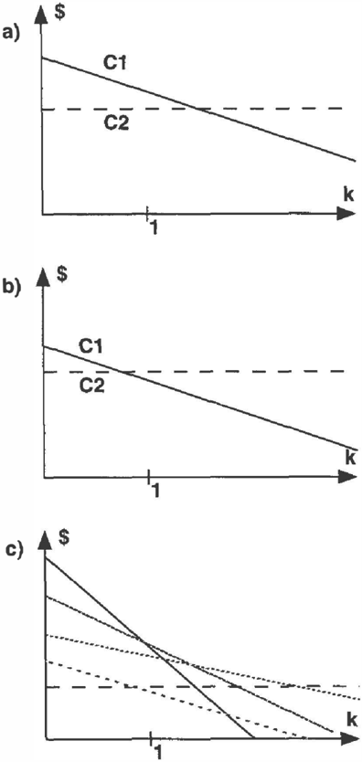
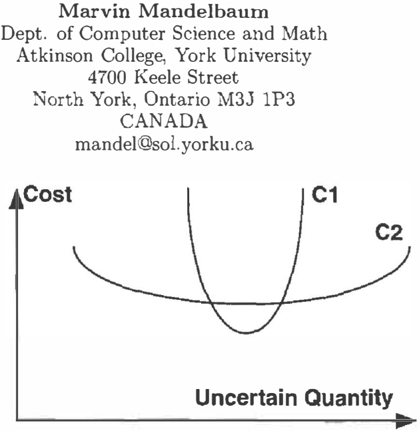
An early classic work on flexibility is Stigler(1939). This paper compares two potential configurations for the operation of a factory, with two corresponding cost curves, as shown in Figure 1. One curve, C1, can acheive a lower cost, but it is quite sensitive to the un­ certain quantity. The other curve, C2, is less sensitive to the uncertainty, but might cost more than Cl. This is an example of what we call robust flexibility, since our concern is developing a plan that will function well in the face of uncertainty. To analyze Stigler's prob­ lem, it is not enough to know the cost curves; we need a probability d i s t r i b u t i on over the uncertain quantity, too.

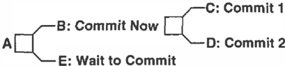
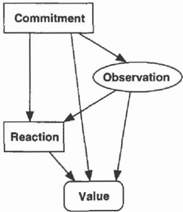
Some more sophisticated approaches to flexibility in­ volve the subtle interaction of information and de­ cisions (Chavez and Shachter 1995; Jones and Os­ troy 1984; Mandelbaum 1978; Marschak and Miya­ sawa 1968· Marschak and Nelson 1962). These frame­ works inv � lve two sequential decisions, a commitment and a reaction, with an intervening obseration, as rep­ resented by the influence diagram shown in Figure 2. Usually some commitments offer more or better reac­ tion alternatives, but at a cost. This is what we call adaptive flexibility, since the flexibility comes from the opportunity to react in light of the observation.

Another school of thought is that decision analysis automatically and implicitly incorporates flexibility (Merkofer 1977). This assumes that we have mod­ eled all of the choices and information available. This approach would subsume both robust and adaptive flexibility, but seems to miss something critical that motivates modelers to consider issues of flexibility in the first place. That is, the decision analytic approach assumes that our model is complete.

In this paper, we follow the decision analysis tradition, but recognize that there is some uncertainty that we were unable to model, perhaps b e c a u s e we could not anticipate it. Reasoning by analogy from the uncer-

tainty we are able to model, we guess how much un­ certainty is "missing" from our model, and we "add" it directly to our value model. This allows us to com­ pare different plans or decision situations, regardless whether they fit the templates for robust or adaptive flexibility. Although the resulting measure is approxi­ mate, it suggests new alternatives we can introduce to increase flexibility.

To illustrate these concepts, consider the management of an investment portfolio. An inflexible investment might be one in which the capital is locked in place for a long term. A robust investment might be in an instrument that performs well in a variety of market conditions. On the other hand, an adaptive investment might be one that can be shifted easily in response to changing markets. Decision analysis provides the machinery for us to explicitly balance the value of this flexibility against any premium in cost. Finally, we might chose to magnify the uncertainty in our decision analysis model, if we believe that there are important uncertainties we have failed to model.

In Section 2 we will explore this concept in more detail. Section 3 develops notation and technical results. We combine those in Section 4 to obtain our definition of flexibility orders and investigate its implications. Fi­ nally, we discuss our conclusions and some directions for further research.

2 CONCEPTS

In this section we describe the concepts behind our approach to flexibility. Coupled with the technical re­ sults in the next section, this leads to the flexibility orders in Section 4.

We can identify several criteria that we would like our approach to satisfy. First, we would like it to operate

on a large variety of general decision models. Ideally, it should be applicable to models represented by the decision analysis type of decision trees (Raiffa 1968) or influence diagrams (Howard and Matheson 1984). Second, it should be conceptually simple. Third, it should be useful for suggesting or stimulating the gen­ eration of new plans or alternatives. Fourth, it should be general enough to incorporate most of the concepts currently in the literature. Fifth, it should agree with our common sense; for example, adding a new alter­ native to a plan should never decrease its flexibility.

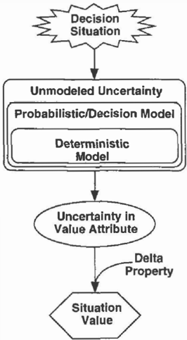
We believe that there is an underlying theme behind the concepts of flexibility in the literature, namely, that a plan must be able to perform well under unan­ ticipated or unmodeled uncertainty. Consider the flow chart shown in Figure 3. Under any decision situation, we can model the performance of a system with vary­ ing degrees of accuracy. The simplest model might be deterministic; we can acheive more accuracy by con­ sidering uncertainty. Regardless, there will be con­ siderable uncertainty that remains unmodeled, either because it was too complex, or because we could not anticipate it.

One challenge is how to recognize and estimate this unmodeled uncertainty. It is difficult to incorporate it into the model, but since all we really care about is the uncertainty in the value attribute, we don't need

to add the uncertainty to the model. Instead, we di­ rectly manipulate the value attribute distribution to incorporate the uncertainty we believe is missing from the model. Finally, if we have additional structure in the value model, as assumed in the next section, we can simplify the analysis of the value of the decision situation.

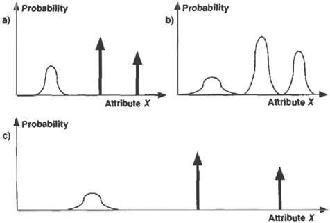
There are a couple of ways we can introduce un­ certainty into the value attribute distribution. Con­ sider the probability distributions over value attributes shown in Figure 4. The modeled distribution in shown in Figure 4a. A natural way to introduce uncertainty into the value distribution is to add independent uncer­ tainty to obtain the distribution shown in Figure 4b. Note that the probability masses become densities, and the the density becomes more diffuse. Another transformation is to rescale the attribute axis to ob­ tain the distribution shown in Figure 4c. In this case, probability masses stay masses but densities become more diffuse.

This approach is based on several key assumptions. First, we can make up for the unmodeled uncertainty by adding some to the model. Second, we can use the uncertainty in the model as a guide for where to add the additonal uncertainty. Third, the model is robust enough to provide sensible outputs when it is distorted beyond its designed range. These assump­ tions are hard to justify, but reasonable if we are to exercise the model to handle the unforeseen. Keep­ ing them in mind, we can recognize that perhaps the most valuable use of the flexibility measure might be in inspiring the generation of new alternatives, that is, suggesting superior plans.

3 NOTATION AND ANALYTICAL RESULTS

In this section, we introduce fundamental concepts of decision-making and the characterization of the value of an uncertain decision situation. We derive a new, simple, and useful result that will allow us to recog­ nize flexibility orders for particular types of decision­ makers.

The decision-maker takes actions that affect her world in uncertain ways, and she chooses actions by compar­ ing their anticipated effects. Bayesian decision analysis provides a coherent rational framework for analyzing her choices. This is not a descriptive technique pre­ dicting the behavior of the decision-maker in practice, but rather a normative approach consistent with a set of conditions that she might reasonably choose to sat­ isfy.

A decision is an irrevocable allocation of resources, usually framed as the selection of an element from a set of possible choices called alternatives. To be a de­ cision, the choice has to be available to the decision­ maker, and it has to be a real commitment. If she can change her mind at no cost she has not yet made a de­ cision. Conversely, if the choice has not yet been made officially, but there is an informal understanding that would make it c o s t l y to change, then a decision has been made already. This corresponds to the flexibility with respect to observations in Merkofer(1977 ) .

After making her choice, the decision-maker faces an uncertain future. She can analyze any possible situa­ tion by considering each possible state and assigning it a von Neumann-Morgenstern utility u, such that if two situations have uncertain utilities ul and u2, re­ spectively, she would prefer the former if and only if E{UI} > E{U2}.

In this paper, we assume that she can also characterize her future in terms of a single variable or attribute of the problem. Her beliefs about the uncertain attribute X we will call her prospect. The most common single attribute is money, although other attributes might be more appropriate for particular problems, such as the probability of successful mission completion for an intelligent agent. Nonetheless, for simplicity the rest of the paper assumes that the single attribute is money.

If the decision-maker is always willing to place a mon­ etary value on any prospect, she is said to have a monetary equivalence for prospects. If she has a mone­ tary equivalence, there is some function $( u) called the willingness to pay, defined as the most she would pay to have a prospect with utility u. Assume that $(u) is strictly increasing, so it has a well defined inverse function, us($), the utility for money.

A decision-maker with monetary equivalence is said to satisfy the delta property if, for any uncertain mone­ tary prospect X and constant payment c,

In that case, she is willing to pay $(u2)- $(ul) money to go from a prospect with utility u1 to a prospect with utility u2. The delta property greatly simplifies calculations of monetary equivalence, but it also im-

plies some strong restrictions on $(u) and u$($). The followi ng theorem is well known (Pratt 1964) and fun­ damental to our analysis.

Theorem 1 (Delta Property) Given a monetary equivalent decision-maker with a utility function for money U$ ( x) that is twice continuously differentiable and u$(x) > 0 , she satisfies the delta property if and only if her absolute risk-aversion is a constant r and

assuming, without loss of generality, that u$(0) = 0 and u$(1) = 1. The more general class of utility func­ tions, given by a+bu$(x) where b > 0, reveals the same preferences among prospects for all choices of a and b.

If she satisfies the delta property, the decision-maker's attitude toward risk is characterized by her constant absolute risk-aversion, r = -u$(x)/u$(x). Her willing­ ness to pay for any uncertain monetary prospect X is called her certain equivalence for X, CE(XIr), and it is defined as

In general, it is different from the expected value of the prospect, E{ X}, and they are related by the ap­ proximation,

which is exact when X has a Gaussian (or normal) distribution. If she is indifferent between any prospect and its expectation then r = 0 and she is said to be risk-neutral. If she never prefers any uncertain mon­ etary prospect to its expectation then r > 0 and she is said to be risk-averse. In general, concave utility functions are risk-averse and linear utility functions are risk-neutral. Using Theorem 1, we can simplify the certain equivalence formula as follows.

Theorem 2 (Certain Equivalence) Given a mon­ etary equivalent decision-maker satisfying the delta property with risk-aversion r > 0 and any uncertain monetary prospect X,

Proof:

For the comparison of flexibility among decision sit­ uations, we would like to characterize the decision­ maker's willingness to pay for prospects after a linear transformation. This can be done simply when the decision-maker satisfies the delta property.

Theorem 3 (Linear Transformation)

Given a monetary equivalent decision-maker satisfy­ ing the delta property with risk-aversion r, independent uncertain monetary prospects X and Z, and positive constant k,

Proof:

As a result of Theorem 3, we have a simple rule for comparing linearly transformed prospects when the decision-maker satisfies the delta property.

Corollary 1 (Transformation Comparison)

Given a monetary equivalent decision-maker satisfying the delta property with risk-aversion r, uncertain mon­ etary prospects X and Y, uncertain monetary prospect Z independent of X andY, and positive constant k, she prefers prospect kX + Z to kY + Z if and only if CE(XJkr) > CE(Yikr).

4 FLEXIBILITY ORDERS

We are now ready to state precisely what it means for one decision situation to be more flexible than another. In this section, we assume that the decision-maker is monetary equivalent satisfying the delta property with risk-aversion r > 0. In that case, we can apply the re­ sults of the previous section to the concepts introduced earlier to obtain a rule for comparing situations. We explore the properties of this rule and show that it satisfies many of the desiderata we identified earlier.

Our approach to comparing decision situations is to attenuate the uncertainty in the prospects X and Y by varying a parameter k. As k increases from 1, the uncertainty in the value distribution is magnified. Two kinds of uncertainty can be added to the distribution, an independent uncertainty and a rescaling of the at­ tribute scale, as shown in Figure 4. Given an uncertain monetary prospect Z which is independent of X and Y (but might depend on k), we transform X to kX + Z to compare flexibilities. The decision-maker consid­ ers X more flexible than Y if she prefers kX + Z to

kY + Z for all k � 1. If she satisfies the delta property, the effects of these changes are easy to analyze, using the results in Corollary 1. Adding uncertainty seems natural, but doesn't change her relative ordering over situations. Rescaling the attribute does change her or­ dering, by effectively rescaling her risk-aversion. These results are incorporated into the following definitions.

Given two uncertain monetary prospects X and Y, a monetary equivalent decision-maker satisfying the delta property with risk-aversion r > 0 is said to find X (strictly) more flexible than Y if there is some pos­ itive K > 0 such that

She is said to find that X (strictly) dominates Y in flexibility if she finds that X is (strictly) more flex­ ible than Y with K = 1, that is,

By this definition, if X (strictly) dominates Y in flex­ ibility then X is (strictly) more flexible than Y.

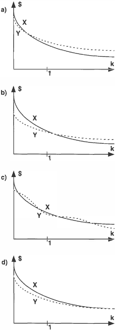
Consider the graphs shown in Figure 5. In Figure 5a and Figure 5b, the uncertain monetary prospect Y is strictly more flexible than the uncertain monetary prospect X, while in Figure 5d, X is more flexible than Y, but not strictly. There is dominance shown in Fig­ ure 5a, where Y strictly dominates X in flexibility, and Figure 5d, where X dominates Y in flexibility. There is no dominance shown in Figure 5b. It is quite possi­ ble to have curves like those shown in Figure 5c, where neither X nor Y is more flexible, and thus neiher can dominate.

Most of the properties of the flexibility compari­ son follow from properties of the certain equivalent, CE(XIkr). The certain equivalent is in units of an at­ tribute, which we have assumed is money. As a func­ tion of k, CE(XIkr) is continuous and nondecreasing (assuming r > 0).

If X is deterministic, that is, it takes on a value for certain, then CE(XIkr) = CE(XIr) for all k > 0. The worst case for X, the smallest possible value of X, is approached by CE(XIkr) as k increases. More for­ mally,

Therefore, if X and Y are two monetary prospects between which the decision-maker is indifferent and Y is deterministic, then Y dominates X in flexibility.

We can now return to the desiderata from Section 2 to see (surprise! surprise!) that they are satisfied by the proposed approach. It is conceptually simple and can be applied to a wide variety of decision models, including decision trees and influence diagrams. In fact, it can even be applied to compare the flexibility at different nodes in the same decision tree. Since the certain equivalent never decreases when an alternative is added, it satisfies our intuition in that flexibility

does not decrease in that case. Of course, it allows the decision-maker to test new alternatives easily and might help her conceive of them, too.

What remains to be shown is that this approach is general enough to incorporate most of the concepts of flexibility in the literature. This follows from the de­ cision analytical nature of the approach. Consider the notion of robust flexibility introduced by Stigler(1939) and illustrated in Figure 1. As k is increased we would expect that the certain equivalent for the situation with cost curve C1 will decrease more rapidly than the situation with cost curve C2. Thus, we obtain the intuitive result that C2 is strictly more flexible than C1, although not necessarily dominant.

Consider the adaptive flexibility case represented by the influence diagram shown in Figure 2. For each possible decision strategy there is a flexibility curve, and we might expect some curves to be more flexible than others. Often these will be the most ad ap tive plans, but it is quite possible that a robust plan could be the most flexible. Thus we can represent adaptive flexibility but we are not restricted to it.

Another example of flexibility comparison corresponds to the sequential decision tree shown in Figure 6. De­ cision B lets us choose between decision C or decision D, so the certain equivalent at B is at least as big as the certain equivalent at either C or D for all k. Therefore, B dominates both C and D in flexibility. By the same logic, A dominates B, C, D, and E in flexibility. If there is no cost to waiting to commit, then E dominates B, C, and D in flexibility.

The analysis is further simplified if the uncertain mon­ etary prospect X is distributed with a Gaussian dis­ tribution, characterized by its mean, E{ X}, and vari­ ance, Var{X}. In this case, the certain equivalent CE(XIkr) is linear ink,

Note that the certain equivalent is unbounded as k increases unless the prospect is deterministic. That is because there is probability mass at arbitrarily low val­ ues, so the worst case certain equivalent is unbounded.

If, in the Stigler example, the monetary prospects C1 and C2 have Gaussian distributions, then they might be represented by the graphs in either Figure 7a or Figure 7b. In both cases, C2 is strictly more flexible than C1 and in Figure 7b C2 strictly dominates C1 in flexibility. Similarly, if every monetary prospect in the adaptive example has a Gaussian distribution, then it might be represented by the graph in Figure 7c. If one curve has a flatter slope than another then it is more flexible. There can be a number of curves that are optimal for some k, but some of the curves might not be optimal for any k.

5 CONCLUSIONS AND FUTURE RESEARCH

In this paper, we have proposed a simple decision­ analytic approach to comparing the fl e x i b i l i t y of di f ­ ferent plans or decision situations. This is particularly useful for automated reasoning tasks where we have limited resources for model construction and analysis (Horvitz 1990). Under such circumstances, we need a robust estimate of the uncertainty which has gone unmodeled, precisely what our measure of flexibility provides.

Our approach behaves according to our intuitive no­ tions of flexibility as well as the concepts in the lit­ erature, without imposing severe restrictions on the types of models. Because the method forces a model beyond its design parameters, it can introduce addi­ tional modeling inaccuracy. Therefore, the "stretched" model should not be examined too precisely, but rather used for the critical c r e at i ve task of stimulating and generating new, more flexible alternatives.

A natural direction for future research would relax the assumption that the decision-maker satisfies the delta property. To increase the uncertainty in the value attribute distribution as a function of parameter k, we could transform the uncertain prospect from X to kX + Z where Z is an uncertain prospect which is in­ dependent of X, although it could depend on k. It is just not clear to us at this point what would be an appropriate value for Z. If a deterministic value were chosen for Z, then this approach would be easy to perform for general decision problems.

The proposed framework looks at different plans as we increase k from 1. Some further research might inves­ tigate the value of considering values of k less than 1. There might even be some insights to be gained by considering negative values of k, turning the decision­ maker into a risk-seeker.

In this paper we have assumed that the decision­ maker is risk-averse, but we could imagine modeling the behavior of a risk-neutral decision-maker, that is a monetary equivalent decision-maker satifying the delta property with absolute risk-aversion r = 0. This poses a couple of problems for our approach. First, there would be no sense in applying the method without any modifications, since CE(X\Ok) = CE(XIO). Second,

in building a model for a risk-neutral decision-maker, there is no need to introduce much of the uncertainty, since it is not relevant for making the decisions. Thus such a model would be quite brittle with respect to changes in r.

Acknowledgements

We benefited greatly from the comments of the anony­ mous referees and many c o l le agues , most notably James Matheson, John Mark Agosta, and Thomas Chavez.

References

Chavez, T. and R. D. Shachter. "Decision Flexibil­ ity." In Uncertainty in Artificial Intelligence: Proceedings of the Eleventh Conference, eds. P Besnard and S Hanks. 77-86. San Mateo, CA: Morgan Kaufmann, 1995.

Horvitz, E. "Computation and Action Under Bounded Resources." PhD thesis, Stanford University, 1990.

Howard, R. A. and J. E. Matheson. "Influence Dia­ grams." In The Principles and Applications of Decision Analysis, eds. R. A. Howard and J. E. Matheson. II. Menlo Park, CA: Strategic Decisions Group, 1984.

Jones, R. A. and J. Ostroy. "Flexibility and Uncer­ tainty." Review of Economic Studies 11 (1984): 13-32.

Mandelbaum, M. "Flexibility in Decision Making: An Exploration and Unification." PhD, Department of Industrial Engineering, University of Toronto, 1978.

Marschak, J. and K. Miyasawa. "Economic Compara­ bility of Information Systems." International Eco­ nomic Review 9 (2 1968): 137-173.

Marschak, T. and R. Nelson. "Flexibility, Uncertainty, and Economic Theory." Macroeconomic 14 (1962): 42-58.

Merkofer, M. W. "The Value of Information Given Decision Flexibility." Management Science 23 (7 1977): 716-727.

Pratt, J. W. "Risk Aversion in the Small and in the Large." Econometrica 41 (1964): 35-39.

Raiffa, H. Decision Analysis. Addison-Wesley, 1968. Reading, MA:

Stigler, G. "Production and Distribution in the Short Run." Journal of Political Economy 47 (1939): 305-329.