A PROBABILISTIC MODEL FOR SENSOR VALIDATION

P.H. lbargiiengoytia Institute de Investigaciones Electricas, A.P. 1-475 Cuernavaca, Mor., 62001, Mexico [email protected]

L.E. Sucar

Institute Tecnologico y de Estudios Superiores de Monterrey Campus Morelos, A.P. 99-C Cuernavaca, Mor., 62050, Mexico [email protected]

Abstract

The validation of data from sensors has be­ come an important issue in the operation and control of modern industrial plants. One ap­ proach is to use know ledge based techniques to detect inconsistencies in measured data. This article presents a probabilistic model for the detection of such inconsistencies. Based on probability propagation, this method is able to find the existence of a possible fault among the set of sensors. That is, if an er­ ror exists, many sensors present an apparent fault due to the propagation from the sen:. sor(s) with a real fault. So the fault detection mechanism can only tell if a sensor has a p o ­ tentwl fault, but it can not tell if the fault is real or apparent. So the central problem is to develop a theory, and then an algorithm, for distinguishing real and apparent faults, given that one or more sensors can fail at the same time. This article then, presents an approach based on two levels: (i) probabilistic reason­ ing, to detect a potential fault, and (ii) con­ straint management, to distinguish the real fault from the apparent. ones. The proposed approach is exemplified by applying it to a power plant model.

1 INTRODUCTION

Computing is playing an increasingly important role in domains like communications, medicine, and industry. Examples of industrial applications include the control of advanced manufacturing plants, power generation, power distribution, and chemical processes. These ap­ plications require the utilization of several method­ ologies that have emerged from the area of artificial intelligence (AI). In general, AI methods are moving towards more realistic domains that require coopera­ tion between several fields of research. This paper de­ scribes an ongoing research project in the utilization of AI methods to solve the problem of sensor valida­ tion. Although the techniques presented here can be

S. Vadera University of Salford Dept. of Mathematics and Computer Science Salford, M5 4WT, U.K. S. [email protected]. uk considered as general, the specific application is in the power plants domain.

The approach proposed in this paper has two layers:

• a prediction layer: which is used to predict the ex­ pected values of the sensors and identify potential faults;
• a constraint satisfaction layer: which is used to distinguish the faulty sensor(s) from the appar­ ently faulty ones.

Both layers make use of a probabilistic network model. A probabilistic or Bayesian network [Pearl, 1988] is a directed acyclic graph (DAG) whose structure corre­ sponds to the dependency relations of the set of vari­ ables represented in the network (nodes), and which is parameterized by the conditional probabilities (links) required to specify the underlying distribution. In this case, the nodes correspond to the sensors that consti­ tute the model. The structure of the network makes explicit the dependence and independence relations between the variables.

In this approach, with the use of probability propaga­ tion, a prediction is made of a variable's value based on other parameters. If this predicated value devi­ ates from the actual value given by a sensor, by some predefined margin, then some fault can be assumed. But the fault detection mechanism can only tell if a sensor has a potential fault, but it can not tell if the fault is real or apparent. The central problem is to de­ velop a theory, and then an algorithm, for distinguish­ ing real and apparent faults, considering that one or more sensors can fail at the same time. For this, the structure of the model is considered, which produces a set of constraints that has to be solved to determine the faulty sensor( s). This article then, presents an ap­ proach based in two levels: (i) probability propagation, to detect a potential fault, and (ii) constraint manage­ ment, to distinguish the real faulty from the apparent ones.

The paper is organized as follows. Section 2 in­ troduces the problem and summarizes previous ap­ proaches. Section :3 presents the approach with the

aid of a si m pl e exam p l e . Section 4 p r e se n t s the ideas formally. S e ct i o n 5 describes a real e x a m p l e that shows the c o mpl e t e technique. Finally, section 6 pr e sen t s the conclusions a n d f u t u r e w o r k .

2 SENSOR VALIDATION

The validation of d a t a from sensors has b e co m e an i m p o rt a nt issue in the operation and control of modern industrial plants. Usually, the control system can not detect s ig ni fi ca nt deviations from the e x p ec te d va l u es g i v e n t h e d es i g n working point, for example of the gas t urb i n e in a p o w e r plant. Conversely, an experienced o pe r a t o r is c a pa b l e of detecting such deviations of a variable by direct observation of the r e la te d v a r i ab l es a n d c on se q u e ntly , avoids false p l a nt t r ips. T h i s p ro j e ct proposes the m ode ll i n g of the operator's experience in the d e t e c t i o n of s e n so r f a i l ur e s .

Typical solutions to this problem, particularly in criti­ cal sy s t e m s where s e c u ri ty is essential, include the use of:

• Hardware redundancy and majority voting: where h a r d ware is d up l i ca t e d and a voting a l gorith m is used to exclude faulty sensors. This is possible in applications such as civilian aircraft or part of the nuclear industry [Yung and C l a r k e , 1989]. How­ e v e r , f o r m an y in du s tr i a l p l a n t s , t h e s e te c h n i q ues are not f e asi b l e wh ere , f o r e x a mp l e , adding fur­ ther se n s o r s might w e a k e n the walls of the pres­ sure vessels.
• Analytical redundancy: in which all process, actu­ at o r s and sensors are monitored c e n t r a l l y . Exam­ ples of these te c h ni q u es are generalized likelihood ratio (GLR) [ Willsky a n d Jones, 1976], a n d failure sensitwe filters [ Massoumnia, 1986].

H owe v er , these a p p r oac h e s can require the develop­ ment of mathematical or knowledge b a se d models whose solution require expensive computer power. Ad­ d iti o n a lly , they are very e x p en s i v e and d e m a n d an e n o rm o us amount of expertise to use them in a differ­ ent p ro c es s or even make a m o d ifi c at i o n of the mon­ itored system. Modern techniques, from where this project is m oti v a t e d , include a decentralised and hier­ archical ap p r o ach [ Yu ng and Clarke, 1989]. A surv e y of some of these techniques can be found in [ B ass e v ill e , 1988].

Previous stages in the d e v e l o p m e nt of this p ro j e c t in­ c l u d e d some experiments in the v a l i d a t i o n of signals in power plants [ I ba r g i i e n go y ti a et al., 1995]. These experiments were b a s ed on the f o l l o w i n g assumption: each sensor is v a l i d a te d in d e p e nd en t l y , i.e., each v a r i ­ able was c o n sid e r ed as the h y p o t h e s i s while some other variables were considered as correct evidence. How­ e v e r , a real solution of the p r o b l e m requires a d iff e r en t set of as s u m p ti o ns to be taken. For example, if the turbine velocity is validated u t ilizi n g only the signals of t e m pera t ur e and pressure, and if the r e as o ni n g re- ports a f a u lt y sensor, it is im p o ssi b l e to define which sensor was the faulty one. In t h i s exa mp l e , if t h e tern­ perature sensor fails and it is u t i l i z e d to d e t e c t a fault in the velocity, the system will certainly report a fail­ ure on the vel o c i t y r e a d in g . This could be a wrong c o nc l u s ion .

Such an a pproa c h , o f c o u r s e , req u i re s the help of do­ main experts to identify the dependencies of the vari­ ables and must also take into account of t he f ol l ow i n g c h a r a ct e r i s t i c s :

• The sensors can provide e rr o ne o u s i n f o r m a t i o n .
• I n fo rm a t i on is available all the t i m e , i . e ., all sen­ sors can be observed as evidence or considered as an h yp o t h e s i s at any t im e .
• The system m u s t r esp o n d within a real time en­ vironment.
• The a p p l i c a t io n considers the possibility of mul­ ti p l e f a u lt s .

3 THE APPROACH PROPOSED

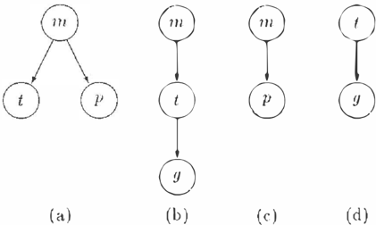
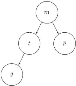
This section presents the ap p r o ach proposed through a very si mp l e e x a m p l e . Assume the model of the gas turbine in a power plant sh o w n in Fig. 11 . The root node m represents the r e a d i n g of the Megawatts gen­ erated in the p l a nt . The temperature is represented by node t and t h e pressure by p. F i n a l l y , g r epr e sen t s the f u e l supplied to the combustion chamber. The val­ idation p r o c e ss s t a r t s a ss u m i n g that t h e sensors, one by on e, are suspect. By probabilistic reasoning, the system d e c i d es if the reading of the sensor is c o r r e c t based on t h e values of the m o s t related variables. This process is carried out for each one of the variables that is r e qu i r ed to be validated. The most closely related

variables for each sensor consist of the Markov blanket of t he sensor variable. A Ma r k o v blanket is defined as the set of variables that make a var i abl e i n de p e nd e n t

1This is a simplified model of the gas turbine. The directions of the arcs do not imply causality.

from t h e others. In a B a y es i a n network, the follow­ ing t h r ee sets of neighbours is su ffi c i e n t for f o r m i n g a M a r k o v blanket of a n o d e : the s e t of d i r e ct. prede­ c e s so r s , direct successors, a n d the d i r e c t predecessors of t h e successors (i.e parents, children, and spouses). The set of v a r i a b l e s that co n s t i t u t e s the Markov blan­ ket of a variable can be seen as a p r o te c ti o n of this variable against. c h a n g e s of v ar i a b l e s outside the blan­ ket. Tlus rnea.ns that, in or d e r t.o analyze a variable, it is o n ly needed to k no w the value of a l l variables in its blanket. For exarnple, in Fig. l a Markov b l a n k e t of t is { m, g}, while a blanket of g consists of { t} only. T a b l e l shows the M a r k o v blankets of each one of the variables in the rnodel of Fig. 1. Considering these

Table I: M a r k o v blankets of the t ur bi n e rnodel.

process variable	Markov blanket
m	{t,p}
	{m,g}
p	{m}
g	{t}

blankets, probabilistic r e a so n i n g is performed utiliz­ ing the re d u c e d rnodels for each variable as s h o w n in Fig. 2. In (a), the equivalent rnodel of m is s h o w n where t h e absence of g i nd i c a t e s that this variable is out. of m.'s Markov blanket.. ln (b), the m o d e l to pre­ dict t indicat.es t.hat thf:' c h a n g f:' s of pare n o t r o n s i c l f:' r e d g i w n a value of m. The sanw for p a n d gin (c) and (d).

7

0

F i gu r e 2: E qu i v a l f:' n t models for the variables. (a) for m, (b) for f. (c) for p, and (d) for y.

A�sunH' t h a t. the tf:'lnpera.ture sensor suff e r s catas­ t.roplllr d a nmge . e.g., thP wires wert> cut.. Starting the Validation jli'UfPSS with Ill, Slllrf:' f jJarftcipafCS i l l the v a l i da t iOn [se<' Fig. 2(a)], an d due to the f a . i ht r f' Ill t, the rPasoning will indicate that. there is a. f a i l u r e in m. Next., thP validation for t wi ll of c o u r s f' indicat.P tlw existence of a f a i l ur P . Tlw v a l i d at i o n uf p w i l l incli­ cat.e> t h a t . this ���n,;or is working p r ope rl y . Finally, t.he validation of !f, g i v en tt.s Pquivalent. rnodel shown in Fig. 2( d), will abo indic<t.t<:> a f a il u r <:> in the sensor Su.

even after the probabilistic reasoning, t he r e is s ti l l con­ fusion: which are real and which are apparent faults?

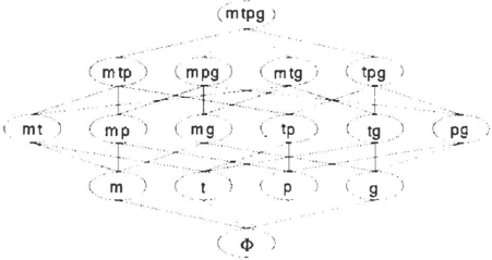
The use of a constraint satisfaction sy s t e m is r e q u ir e d . In th i s case, the presence of a faulty sensor causes a constrained area of rnaniff:'st.ation whi c h forms a con­ text. The c o n t e xt s can be a r r a n g e d in a lattice as s how n in Fig. : ) . The lo w e r nod!:' represents the no fault contf:'xt of t.he s y s t e r n . The upp!:'r l a y e r s repre­ Sf:'nt an incremental assumption of f a u l t y sensors. The t o p node represents a co nt e xt . where all the Sf:'nsors are reported f a u l t y .

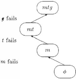
Every step in th e probabilist.ic r f:' a s on i n g generates a constraint. for the final d e t ec t i o n of the sensor in fail. S t a r t i n g at the bottom of the lattice of F i g. 3, eac-h step will rnake a t ra n s iti o n between thf:' n od e s of the lattice. Figure 4 s h o ws the transitions from thP b o t t o m node (cp) to thf:' final n o d e : {m,l,y}.

This papPr s h o w s that there exist.� a correspondence between a fault in a sensor and the n o d e of the lattice o b t a in e d when propagating the failures r e p o r t e d by the probabilistic reasoning. In this e x a rn p le , when t fails. the rorrt>sponcling !attic!:' node is { m, t, y}. This uode c or r e s p o n d s to th� set. of variables that f o nns the Markov blanket. of a v a r i a b h ' plus tlw variable its e l f.

Tablt> :l :sl!ow,; tlw Markov blankets and the lattice's nodt' cont>spmHling to t.llt' constrctints p r o p a g a t i o n for t'ach variable> in fanlt. Tht'u. if a propagation on the lattice finishes in { m, t, p} it signifies that the fault. is in s e n s o r m. L a t t i ce node { m, p} c o r r e s p o n d s to p, and finally, { l. !I } co r r e s p o n d s to y.

Table 2: Markov blankets of tht> simple turbine m o d e l

.

proct>:s� variable	Markov blanket	lattice node
m	{t,p}	{m,t,p}
	{in,g}	{m,t,g}
p	{m}	{m,p}
!I	{t}	{t,g}

With this llH'chani:ml, e v en if t he r e exist rnany appar­ e n t faults. t.he p r o p a g a t i o n on t.ht> l a t ti ce distinguishes w hi c h setJsor wnt.ains t.ht> re a l fault.. Table 2 consid­ ers only single f<wlts. However, thf' method assures that if tlw latt.irf' propagation finislws in a n od e not inrluded in Table 2, it. signifif's t h a t . tiH're exist.;; mor" than one sensor with a fault. S e c t i o n 4 explains and demonstrat.f's t.hf'st-· JllPChanisrHs.

4 A THEORY FOR SENSOR VALIDATION

Tlw prob;dJilist.ic: JJ ILHit'J fur ,;ellsur vaJid;d.iuu rurJ:sisC:-; of a Bayesian Hf't.work as dt>tint>d by Pearl [Pf'arl. 19H8]. That is, a directed ar.ydic graph (; which is a mmimal !-map of tlw dt>pend<·ncy n w d el M for a probability distribution P. (; is an !-map or mdcprndcncy map of M if

wherf' I(X,Z, Y), X, y·,z art' subsets of V, denot.es conditional independt>nce of X and Y given Z, and < X I Z / Y >t) rt>present.s a graph (,'where tht' sub­ set. Z of nodPs in t e r ce p t s all paths betwPen t.he nod.Ps of X and thust> of r'. U is an !-map of M if every conditiunal indt>pPtHiencf' nmdit.ion (according t.o tht' D-sr:pnmliun criteria) d i� p l a y f' d in (; rorresporids t.o a va l i d cuudit.iunal indt'peuclenct> rflationship in lvJ. It is a 11/.lll.lll/.a/ !-map if uunf' of tt.s lillh rau bt> deiPt.ed wit.ltuut dt>struyirtg it:; 1-lll.!lJil!ts.� [F't>Ml. lDt!H].

Dt>tiuitiou 1: (;iVPII a pruhahilit.y di�t.rihutiuu P u11 a. st'l uf variah],·,.; V. aDA(;(;= (1/, E) (I" is a Sf>t. of nuciP:>, t_· is a st>l uf link�) is C\. Ba:ljcswn Ndwu·rl.: iff(; is a minnnal!-m!lJI of P.

A Mnrkuv blrwktl. for a.uy node X in a B a y e si a n net­ w o r k is it suh:-;t>t of V w h i c h rnakes it. i n de p e nd e n t frorn tilE' ut.lwr variahlt>s.

Definition 2: A M (u·kun (J{anl.:et M H( X) of any vari­ able X E V is <l su hst>l. .'->' C \/ w herf' X rf. S for w hiC"h

In a Bayesian n e t w o r k , the Markov blanket of a node X can b e formed by the union of its d i r ec t parents P A(X), its d i r ec t successors .')U(X), and all direct parents of t h e latter S'P(X) (X's spouses). This f o l ­ lows f r om the axioms of rondi tiona! independencl:' and t.lw So1mdnc.5.s theorem [Pearl d al., 1990]. Although there may be o t h e r Markov blankets, only this type of blankets are considered.

In using a Bayesian network representation for sensor validation, the following a s s u m p t ion s are m a d e :

1. Observability: all the variables (sensors) can be measured directly 2.
2. Fault detection: i f there is an error in sensor X it can always be detected. T h a t is ;r0 -:j:. Xp, w h e r e x0 is t h e observed value, and a:P t h t> predicted value. The predicted value is the one with highest prob­ ability obtained by probability p ro paga t i o n from its neighbours, M H(X), assuming X is unknown. This is c a l l e d a real fault denoted by Fr( X).
3. ;3. F a u l t propagation: if a sensor Y has a re al fault Fr(Y), andY EM B(X), a fault in X w i ll be de­ t e c t e d , that is a:0 =/= Xp. This is called an apparent fault denoted by Frt(X). In general, Y c o u l d he a set of sensors such that Y C (; .

If a sew;or (variable} X ha, a rPal fault and / or appar­ e n t fault then it is called a potmtial fault Fp(X). Th<> f a u l t detection mechanism can o n l y tell if a sensor has a p o t ent i a l fault, but (without considering other s e n ­ »ors) it can not tell if t h e fault. is rPal or apparent. So the central problem is to d Pv e l o p a th e o r y. and then an al g o r i t h m , for distinguishing real and apparent faults, considering t h a t one or more sensors can fail at the same time.

Lemma 1 (symmetry): Let. X bt-> a node in a Ba y e s i a n network G wi t h a Markov blanket.:J M H(X), X E M H(Y;) iff Yi EM B(X), 'v'Y; E G. That is, X is i11 t h e Markov blanket of all the variables t ha t are in M B(X), and it is only in these Markov blankets.

Proof: First. the proof that. if Y EM B(X) then X E ll1 B(Y). (;iven t h at M H(X) = PA(X) u S'U(X) u S'P(X), tlm1 Y E PA(X) or Y E SU(X) or Y E ,<..,'f'(X), so X E Slf(Y) or X E P A(Y) or X E SP(Y), respectively. ln any ca.sf'. X E J'vl H(Y). Next, th e prooft.hat ift' � MB(X) tlwn X rf. MB(Y). By Ddinit.ion 2, !(X. /VI B(X). ( ; - M B(X)- X), and by thP :-.':ymmdr:q a,nd Drcomposilwn axioms [Pearl d al., 19DO] /(t';, M B(X), X), \iY; E G- M B(X)-X. Thus X is not iu M B(Y).D

."A one to one correspuudence between nodes, variables, and sensors i,; considered.

'This lemma and the subsequent theorems apply to :\1 arkov blankets formed by the direct parents, direct suc­ cessors, and direct parents of the latter.

The atcnded Markov blanket EM B(X) is defint->d as the union between thf:' Markov blanket of a v a ri a b l e and the variable, i.e., EM B ( X ) =XU M B(X).

Theureu1 1: If there is an error in sensor X. i t will p ro d u c e a potcntwl fault in X, and all the s e nso r s in M B ( X ) , and no other sensor.

Proof: From assurnption 2, an error in X produces a potential fault in X. From Lemma 1, X is an el­ ement of the MB of all sensors Y; E M B(X), so by assumption :3, an error in X produces potential faults in all sensors in M B ( X ) . Finally, from Lemma 1 X is no t an elernent of any other MB, so no other potential fault will b e detected (assuming X is the only sensor in f ault.) . O ·

Corollary 1: A s s u m in g a single (only one sensor fails} real fault. a potwtwl fault in all the sensors in 8 C (; implies a real fault in a sensor X such that EM B(X) = S, and X E .)'.

Given t ha t an error in a sensor produees a potential fault. in all the sensors in its EMB and only in those, a potential fault in all sensors in .'J' implies that a sensor in fault has its EM B =,)'(assuming one real fault).

Corollary 2: If all Markov blankets are different in G, M B(Y) =/: M B(Z), V'l, Z E G. Y =/: Z, then all single real faults F1·(X) can he distinguished in G. In this case only the nodes in EM B (X ) will have a potentwl fault.

The validity of Corollary 2 follows from Corollary l and the fa('t that all MB are different.

The pr o b le m is that two or more variables could have the s a rn e Markov blanket. Such is the case of leaf nodes with the same parent in a tree.

Corollary 3: If there is an error i n sensor X with EM B(X), and also an error in Y with EM B(Y), they will p rod u c e potential fault.s in all nodes Z E EM B(X) U Eivf B(Y). ln general, if there are errors in sensors X;, i = 1, .. . , m, they will produce potential faults in all nodes Z E Elvf B(X!} U . . U EM B(Xm)

Corollary ;) follows clire('tly frorn Theorem l. assurning that t w o or rnore Pnors will not cancel e a e h other (i.e., if Z E M B(X) and Z E M B(Y) and b o t h , X and Y f a i l , still a potential fault. will be de t ec t e d in Z).

Theorem 2: If there is an error in sensor X with EM B(X). and Y E EM B(X) with EM B(Y) C EM B(X), and rnultiple faults (more than one sen­ sor can fail sirnultaneously) are considered, then there is no d i s ti nc t i on between Fr·(X) or F1·(X) A F1·(Y)

Proof: By Theoren1 l, Fr(X) will produce appar­ ent faults in EM B(X). Fr(X) A Fr(Y) will pro­ duce apparent faults in EM B(X) U EM B(Y) by C o r o l l a r y :3 So if EM B(Y) c EM B(X}, t.hen EM B ( X ) u EM B(Y) = EM B(X) so both cases are indistinguishable. 0

Theorem 3: Multiple faults can be distinguished if all t he extended Markov blankets of tlw SPnsors with errors are disjoint.

Proof: It follows frorn Corollary 2 and :).0

Theoreu1 4: If the s e t of nodes :-,·with a p p a re n t faults in G is different from all EMB(X;), VX, E G, there must be multiple (at least 2) real faults i n G. T h e sensors X; such EM B(X;) C S' can have real faults, an only these sensors.

Proof: From T h e o r e m 1, a real fault in X produces apparent faults in and only in the set of sensors in EM B(X). So a single fault can not p r od u c e a set S of po t e n t ia l faults different from all EM B in C. F r om Corollary ::1, the sensors whose EM B is a subset of S can be in fault, and by Theorem 1, only these sensors.O

Based on the theory clescri bed above, an algorithm is r e q u ire d so that, once the model has been established, and the Markov and extended Markov blankets have b e e n defined, the detec.tion of real f ai l ur e s can be car­ ried out. The proposed algorithm for sensor validation is the following:

1. Obtain the model (i . e., the Bayesian network) of the application p ro c ess.
2. Make a list of the variables to be validated and build a table of EMB for each variable.
3. :). Take each one of the variables to be checked as the h y p o t h e s i s , instantiate the variables that form the Markov blanket of the hypothesis. and propagate the probabilities to obtain the posterior probabil­ ity of the variable given the evidence.
4. C o mp a re t he pr ed i c t e d value (the po s te r i o r prob­ ability) with the current value of the variable and decide if an error exists.
5. Repeat steps :3 and 4 u n ti l all the variables in the list have been examined and the set of sensors with apparent faults (.':J') is obtained.
6. Compare the set of sensors i n fault obtained in step ,'), with the table of the EM B fo r each vari­ able:
7. (a) If.)' = dJ there a r e no faults.
8. (b) If 5' is e q ua l to the EMB of a variable X, and there is no other EMB which is a subset of s·, then there is a single real fault in X.
9. (c) If .5' is e q u a l to the EMB of a variable X, and there are one or m o r e EM B which are subsets of .':J', t h en there is a real fault in X, and p o ssib ly , real faults in the sensors whose EM B are subsets of .)'.
10. (d) If S is equal t o the union of several EMB and all these are disjoint, there are multiple real faults i n all the sensors w h o s e EM B are i n S.
11. (e) If none of t h e above cases is satisfied, then there are multiple faults but they can not be distinguished. All the sensors whose EMB are subsets of S could have a real fault.

Notice t h a t the propagation on t he lattice is an index­ ing of a, table, i.e., no e<tlc.ulations art' rE>quired . This is a very important feature for a system running in real tirne.

The next. section explains the algorithm proposed in a real example, taken f ro m a t.h�rmoelectrical power plant.

5 SENSOR VALIDATION IN A POWER PLANT

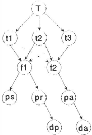
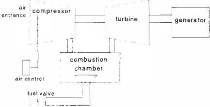
In o r d e r to de r n o n st r a t e the ideas contained in t hi s article, a rnodule of a com bin e d cycle power plant was chosen: the gas turbine. F i g u r e 5 s h o w s a simplified sc he rn at i c dia.grarn of the type of gas turbines at the Dos Bo('as and Gomu Palacio power plants in Mexico.

.,

l

!

A g<ts turbine consists fundamentally o f four main parts: t h e compressor, t h e combustion chamber, the turbin<" itself and tlw ge n e r at or . The corn p r ess o r feeds air to t h e combustion c hamb e r , wheff� the g a s is also fed . Here, the cornhustion produces h i g h pressure gases at high ternJwratun'_ The expansion of t h es e ga�es in tllP t u r b i n P producPs t l l P turbine rotation w i t h � t. o r q ue t hat is transrni ttf'd t o the g en e r a t or in or d e r to produce the dert.rir power output. The ai r is rf'g­ ulat.ed by means of the mlet guzde vanes ( I < � V ) o f the compressor, and a c o n t r o l valve d o c s the same for the ga.'> fuel in tlw combustion charnber. The control valve is cotnrnanded by the control system or by the oper­ a t o r in t h e rnanua.l operation mode, and its ape r t u r e ran be read by a p o s i t i o n sensor. The temperature at the blade p at h . which is the rnost c r i t i c a l variable. is taken along tlw c i rcumf e r e n c e of the turbine.

Among all var i a b l e :s that participate in the gas tur­ bine, only a few are directly 1 ne a sure d by the sensors. Since the blade path temperature is the most critical variable. i t is obtain<'cl t h r o u g h sixteen thermocouple sensors l o cat.Pcl all around the t. u r b i w' . From t h ese sixteen, three �ets of averages arc t a k e n by analog cir­ cuitry. These v a l u es are then a ve r a g ed in order to

obtain a single value for t h e temperature. T h e op� e r a t or is informed of the average temperature, which is also used by a control s t ra t eg y to protect the en­ gine. Table :3 shows the list. of v a ri a bl es of the model of Fig. 6 inc.luding t h e explanation of t h e process variable, their name, and their corresponding Markov blankets. From Table :3, i t is easy to see that t h e l a t -

Table 3: Variables in the example.

process variable	Markov blanket
Selected b l a d e path ternp. 1	{t 1 , t 2, t : 3}
Blade path t e m p . avg.	{T, t2, t:3 , j1 , /2}
Blade p a t h temp. avg. �	{T, t 1 , t:3 , /1, /2}
Blade path temp. avg. :3	{T, t l , t2, / 1 , !2}
Flow of gas	{ t 1, t2, t3, ps, pr}
Flow of a i r	{ t 1, t2, t :3 , pa}
Gas fuel pressure supply	{! 1 }
Real fuel valve p o sit i o n	{!1 , dp}
Real IGV position	{!2, da}
Position d em a n d fuel valve	{ p r}
Position demand IGV's	{pa}

tice nodes for variables t l , t 2 , and t:) i s e x a c tly the s a m e , i . e . , { T, t 1 , t 2 , t :l , fl , f� } . Hence according to section 4, failures a m o ngs t . these sensors c a n not be distinguished by the system.

In this ex am p l e , if t h e node {t l , t 2 , t :l , ps. pr } is o b ­ tained in the propagation on the \attire, according to Table 3, t h e fault is undoubtedly in the sensor m e a ­ suring the variable f l or flow of gas. Contrary to the e x a m p l e of Fig I which is very simple, this e x a m pl e allows the case of multiple faults also to be shown. Suppose that. the sensor of the real fuel valve posi­ tion (pr) fails together with the s e ns or of the p o s i ­ tion dernand of I GVs ( da ) . The lattice node of pr i s { f l , pr, dp} , and the da node is {pa, da}. Conse­ quently, the lattice n o de of the c o m b i n e d failure o f pr and da is the union of t h e i r corresponding lattice nodes, i .e., { f l , pr, pa, dp, da} . Finally, if there exists a fault in sensor dp and sensor p1·, the r e s u l t ing un i o n

between both ('X t (' n de d Markov b l a n k e t o> io> given by {f1 , dp, pr } wltir:h i� exactly the same as thP lat.tir:e nod e uf ]11' _ In t.his c.a.sP , the model can only ensurE' t ha t there exi:-;t:-; a fault in pr but it can not distin­ guish the duuhlt' f a u l t in pt and dp.

6 CONCLUSIONS AND FUTURE WORK

Thi� papPr has p r P � P n t e d an a pp ro ac h to de t e c t in g in­ con::;ist.PnciPs i n tlw r e a d i n g s of sensors in industrial plants. This approach. ba s ed on Bayesian networks and constraint satisfaction , possPsses a l s o tlw advan­ tage that much o f the p r o c e s s i n g IS performed off l ine. i . e . before t h e system operate� in t he plant. This characteristic will h e l p i n t h e real time pe r f o r m a n c E' re­ ttuired in n w s t uf t. h e i ndustrial applications. With the use of prohahili ty p rop a g a t i o n , a prediction is 1nade of a variable's val ue based on other pararnf'ters. [f t h i s predicated V<due dt:>vi<Lt.Ps front the actual v a l u e gi ven by a s e n so r , by solllt ' p r P d e fiu e d rnargin, then som<-' f a u l t can l w assumed. This fault d e t e ct i o n rned1anism can on l y trdl if a sPnsor has a potential fault, b u t it can not tPll i f t lw faul t is real or a p p a r e n t . A tlw­ ory a nd algorithm wPre developed for distingmshmg real and apparent. f a u l t s , considering that one or nwre sensors can fail at the sante time. For this. th e struc­ ture of t l w nwdt:>l i s co n s i d e r P d , which p r o d u ce s a s e t of constramts that. has t o he solved to df'terrnine the faulty sensor(s) . Tlw approach is b a s e d on two IPv­ els: ( i ) probability propagation, to detect a p o t e n t i a l fault , and ( i t ) run:>tt·a.iut managenwnt. to distinguish tht:> real fanlts front dw a p p a r P n t ont:>s. The uwthod w as appliPd to a situplifi,..cl rnodPI of a gas turlHn<-'

The m a i u l i l l l i t a t i u u uf the proposed a l g or i t l uu is t hat i n somP ca:><-'S . i t i::< nut p oss i b l e to i d (' nt ify p rel' isPiy tht· r e a l fault ;uuung all the s e n w r :> with pot('ntial f a u l t s . Tht:> cases wlwn no <-' X<-txt answer is p rov i d e d ar<-' suru­ m a r i z e c l as follows:

• two or 11101'<-' s P n so r s with the same EM B,
• a don hie fault IV lwr<-' onp EM B i s a subset o f t. lw otlwr.
• mtdtipiP f < l u l t s i n which somP of t l w EM B f a. l l m tlw p r e vi o us cases.

For example, in Fig. 6, variablPs t 1 . t '2 , and t:3 fall Pll the fir s t . ca�<-'In Fig. I there is an exarnple of t h e second <ast� . The EMB of p is {m. p } and th e m ' s EMB is {m. p. t} HPr<-', if m a n d p f a i l at t l w same time, this ntt:>chanisrn c a n only infonn that 111 fai!PCI but i t can not. tdl if p f a i l e d or not.

In order t.u bP a pp l ie d in a real p l a n t . , the t.Pchnique rnust address ad eli tiona! issues.

First , thP techniques descrilwd i n t h i s papPr work well whPn thP sPnsor f a i l s cat.astrophirally. HowPwr. a rt:>al p r o b l (' m fac('d by t . l w npPrat.ors i n p ow('r pl ants ts slo w failurPs , . ;uch a,.; d<-'calihrat.ion. DiffPrent probabilistic mechanisms have to be incluclecl in order to dPtect such slow deviations, for example. temporal reason­ i n g . Then, t h e utilization of t P m p or a l probabilistic r eas o n i n g is required at tlw lowt:>r l t:> v d of clPcision .

The use of a probabilistic t e m p o r a l reasoning mecha­ nism, b e s i d e s the slow failures rnent.ioned above, will also help to fonts on the clynarnic characteristics of the rnodels in a p o w e r plant. Since the process of power gFnt:>ration has d i ff P r e n t ph asPs, ( e . g . , st a r t up, s y n ­ chronization, stt:>ady s t a t e , and stop) different proba­ b i l i s t i c rnoclels are required . For exarnple, during the s t a r t u p phase, the v e l oc i t y of the t u r bi n e is the vari­ able that. will be s u b st i tute d by the Megawatts gen­ erated d u r i n g other phases. A m e c h a n i s m that a l l o w s changes in the probabilistic rnodel is required .

[n a d d i t i o n to t he two levels of d Pc i s i o n , a new level of r t:> a s o ni ng is r e q ui rP d to det.Pct when tllf' fault is in tlw process, and not in the readings of the i nst.rmnent.s . For ex a m p l e , thP s e n s o r validat.or may detect an e r ­ roneous r e a d i n g frorn the turbine ve l o c i t y given the temperature and prt:>ssure rneasures. However, it may be the case that t h P r e is a SPrious rnechanical prob­ lem with t h e generator which may cause that the re a l velocity to go to a ve r y low value.

Finally, the l a s t stf'p i n t h e p r o j e c t will be t h e con­ struction of a pro t o t yp e which performs i n a thermo­ e l e c t r i c a l power plant. Th i s pr o t ot y p e r e q u i r es a r ea l time response. F o r this reason, different mechanisms of s c h ed u l in g have to be d ev e l o p ed , e.g . . any tzme al­ gorithrns [ I bargiiengoytia d al. , 1 99.'i].

A eknow ledgtnen t s

Sp e c i al thanks to E du a r d o Morale� who p r o vi d e d Ill­ val u a b l <-' advice i n thP design of tbts nwthodology. Thanks abo t.o the anony mous n>ferees for t h e i r corn­ lll<-' llt.s which improved this artie!<-' This research is supported by a g r a n t from C:ON ACYT a n d l i E unclPr the In-House I I E/SA LFO RD/CONACYT doc­ t or a l p r og r a m m e .

References

• [ Basseville, 1 988] M. Basseville. Detecting c h a n g es i n signals and s y s t ems . A utomatica, 24(:3 ) ::309-:326 , 1 98�.

[l bargiiPngoytia et al. , 1 99.5] P. H . I b argiiengoytia, L. E. Sticar, and S _ Vadera. Real time intelligent signal validation in power plants. In Pr'OC . .'>' e cond I F A (' Sympo.sium on Control of Pow a Plants and Power Sy.strms, pp 1 07- 1 1 2 , Cancun Q.R., Mexico, 1 9 9 5 .

[ Massournnia, 1 986] M.A. M assounmia. A geornetric approa�h to the synthesis of f a i l u r e detection fil­ ters. IEEE Transactzuns on Automatic Control, :� 1 ( 9 ) : 8 :39-846 , 1 986.

[Pearl e l a/. , Hl90] . ) PParl, D. Geig<-'r, a n d T. Verma. ( :ondit.ional independPnce and its representation . I n

• ( ; _ S!Jafer aud .J . Pearl . edit.ur� . Ro<dmgs m fin­ CfT"Iam Rt·asonmg. pafo!;e:'> Gfi- - ( ) 0 . Morgan Kaufmann. San M atPo. Califomia. ( T . S . A . . 1 H90
• [ Pearl , 1 f!KX] .I . Pearl. l'r-u habilzsitc nasunmg m mtd­ ltgfJI I syslrm.-;_ M organ K aufmann, Palo Alto, Calif I'. S A , HJK:-i .
• [ Willsky and .J ont's, lD76] A.S. Willsky and H . L . .J ones. A generalised like­ l i h o o d ratio approach to detPrtion and Pstirnation of j lllll ps in li m·a r systPms. J EEE Tmnsactzon.s on Automattc Cont7'i!l 2 1 ( 2 ) : 1 08 - 1 1 2 , 1 976 .
• [Yung and ( � brkt", l f! KH] S. K . Yung and D . W . ( �Iarke. Loud Sf:'l!Sor validation . M ra.snn:m ent 6! Control, 22P) 1 :32- 1 4 1 . 1 9Kfl .