A scheme for approximating probabilistic inference

Rina Dechter•and Irina Rish

Department of Information and Computer Science University of California, Irvine dechter@ics. uci. edu

Abstract

This paper describes a class of probabilistic approximation algorithms based on bucket elimination which offer adjustable levels of accuracy and efficiency. We analyze the ap­ proximation for several tasks: finding the most probable explanation, belief updat­ ing and finding the maximum a posteriori hypothesis. We identify regions of com­ pleteness and provide preliminary empiri­ cal evaluation on randomly generated net­ works.

1 Overview

Bucket elimination, is a unifying algorithmic frame­ work that generalizes dynamic programming to en­ able many complex problem-solving and reasoning activities. Among the algorithms that can be ac­ commodated within this framework are directional resolution for propositional satisfiability, adaptive consistency for constraint satisfaction, Fourier and Gaussian elimination for linear equalities and in­ equalities, and dynamic programming for combina­ torial optimization [7]. Many algorithms for proba­ bilistic inference, such as belief updating, finding the most probable explanation, finding the maximum a posteriori hypothesis, and calculating the maximum expected utility, also can be expressed as bucket­ elimination algorithms [3].

The main virtues of this framework are simplic­ ity and generality. By simplicity, we mean that complete specification of these algorithms is feasible

Thls work was partially supported by NSF grant IRI-9157636 and by Air Force Office of Scientific Re­ search grant, AFOSR 900136, Rockwell International and Amada of America.

without employing extensive terminology, thus mak­ ing the algorithms accessible to researchers working in diverse areas. More important, their uniformity facilitates the transfer of ideas, applications, and solutions between disciplines. Indeed, all bucket­ elimination algorithms are similar enough to make any improvement to a single algorithm applicable to all others in its class.

Normally, the input to a bucket-elimination algo­ rithm consists of a knowledge-base theory specified by a collection of functions or relations, ( e.g., clauses for propositional satisfiability, constraints, or condi­ tional probability matrices for belief networks ) . In its first step, the algorithm partitions the functions into buckets, each associated with a single variable. Given a variable ordering, the bucket of a partic­ ular variable contains the functions defined on that variable, provided the function is not defined on vari­ ables higher in the ordering. Next, buckets are pro­ cessed from top to bottom. When the bucket of vari­ able X is processed, an elimination procedure or an inference procedure is performed over the functions in its bucket. The result is a new function defined over all the variables mentioned in the bucket, ex­ cluding X. This function summarizes the "effect" of X on the remainder of the problem. The new function is placed in a lower bucket. For illustration we include algorithm elim-mpe, a bucket-elimination algorithm for computing the maximum probable ex­ planation in a belief network ( Figure 1) [3].

An important property of variable elimination algo­ rithms is that their performance can be predicted using a graph parameter called induced width [5}, ( also called tree-width [ l ] ) , which is the largest clus­ ter in an optimal tree-embedding of the graph. In general, a given theory and its query can be asso­ ciated with an interaction graph describing various dependencies between variables. The complexity of bucket-elimination algorithms is time and space ex-

ponential in the induced width of the problem's in­ teraction graph. Depending on the variable order­ ing, the size of the induced width will vary and this leads to different performance guarantees.

When a problem has a large induced width bucket­ elimination is unsuitable because of its extensive memory demand. Approximation algorithms should be attempted instead. We present here a collection of parameterized approximation algorithms for prob­ abilistic inference that approximate bucket elimina­ tion with varying degrees of accuracy and efficiency. In a companion paper [4], we presented a similar ap­ proach for dynamic programming algorithms, solv­ ing combinatorial optimization problems, and belief updating. Here we focus on two tasks: finding the most probable explanation and finding the maxi­ mum a posteriori hypothesis. We also show under what conditions the approximations are complete and provide preliminary empirical evaluation of the algorithms on randomly generated networks.

After some preliminaries ( section 2), we develop the approximation scheme for the most probable expla­ nation task ( section 3 ) , for belief updating ( section 4), and for the maximum a posteriori hypothesis ( section 5). We summarize the results of our em­ pirical evaluation in section 6. Related work and conclusions are presented in section 7.

2 Preliminaries

Definition 2.1 (graph concepts)

A directed graph is a pair, G = {V, E }, where V = {X1, ... , Xn} is a set of elements and E = {(X,,Xi)IX,,Xj E V } is the set of edges. I f (X;, Xj) E E, we say that X; points to Xi. For each variable X;, pa(X;) or pa;, is the 11et of variable11 pointing to X, in G, while the. 11et of child node11 of X,, denoted ch(X,), compri11e!l the variables that X1 point11 to. The family of X;, F,, includes X1 and its child variable11. A directed graph is acyclic if it ha11 no directed cycle11. An ordered graph i!l a pair ( G, d) where G i11 an undirected graph and d = X 1 1 ... , Xn is an ordering of the nodes. The width of a node in an ordered graph i!l the number of the node 18 neighbors that precede it in the ordering. The width of an or­ dering d, denoted w(d), is the maximum width over all nodes. The induced width of an ordered graph, w * (d), is the width of the induced ordered graph ob­ tained by processing the node!l from last to first,· when node X is processed, all its neighbor11 that precede it in the ordering are connected. The induced width of a graph, W*, is the minimal induced width over all it!l ordering!lj it is al!lo known as the tree-width [1].

A poly-tree is an acyclic directed graph whose under­ lying undirected graph (ignoring the arrows) has no loops. The moral graph of a directed gra p h G is the undirected graph obtained by connecting the parents of all the node11 in G and then removing the arrows.

Definition 2.2 (belief networks)

Let X = {X1, ... , Xn} be a set of random variables over multivalued domains D1, ... , Dn. A belief net­ work (BN) is a pair (G, P) where G is a directed acyclic graph and P = {P;}. P; = {P(X,Ipa(X,))} are the conditional probability matrices associated with X,. An a11signment (X1 = :llt, .. . ,Xn = :!l n } can be. abbreviated to :z: = ( :ct. . . . , :c n) · The BN represents a probability distribution P(zt, . . . . , :en ) = n�=lP(:z:, l:z:pa(x,)), where, Zs i!l the projection of z over a sub11et S. if u is a tuple over a &ubset X, then us denotes that assignment, which is restricted to the variables in S n X. An evidence set e is an instantiated subset of variables. We use (us, :cp) to denote the tuple us appended by a value :z:P of Xp, where Xp is not in S. We define i, = (:c1, ... , z,) and i{ = (z;, :z:i+l· ... , Zj).

Definition 2.3 (elimination functions) Given a function h defined over subset of variables S, where X E S, the functions (minxh), (ma:cxh), (meanxh), and CL:x h) are defined over U S -{X} as follows. For every U u, (minxh)(u) mi� h(u, z), (ma:z:xh)(u) m� h(u, :z:), (L:x h)(u) I: .. h(u, :z:), and (meanxh)(u) = L: .. h�ij), where lXI i6 the car­ dinality of X 's domain. Given a 6et of functions ht, . . . , h; defined over the 11ubset6 81, . . . , S1, the prod­ uct function (Tij hi) and L: 1 h1 are defined over U = UjSj. For every U = u, (TI1h1)(u) = TI1hi(us3) and (L: 1 hj)(u) = Lj hj(us;)·

Definition 2.4 (probabilistic tasks)

The mo11t probable explanation (mpe) task is to find an anignment :z:0 = ( :z:011 . . . , :Z:0n ) such that p(:z:0) = ma.x.z,. Ilf=1 P(:c,, el:z:p4;). The belief assessment task of X = :z: is to find bel(:z:) = P(X = :z: l e ) . Given a set of hypothe11ize.d variables A = {At, ... , A�:}, A � X, the maximum a posteriori hypothesis (map) task is to find an as6ignment a0 = ( a01, . . . , a 0 �c ) such that p(a0) = ma.x;,11 L:'".x- A Ilf:::::1P(:z:;l:cpa,, e ) .

3 Approximating the mpe

Figure 1 shows bucket-elimination algorithm elim­ mpe [ 3 ] for computing mpe. Given a variable or­ dering and a partitioning of the conditional proba­ bilities into their respective buckets, the algorithm

Algorithm elim-mpe

Input: A belief network BN = {P1, ... , Pn}; an or­ dering of the variables, d; observations e. Output: The most probable assignment.

1. Initialize: Partition BN into buckeh, ... , bucketn, where bucket; contains all matrices whose highest vari­ able is X,. P u t each observed variable into its appro­ priate bucket. Let S1, . . . , S; be the subset of variables in the processed bucket on which matrices ( new or old ) are defined.
2. Backward: For p +n downto 1, do for h1,h3, ... ,h; in bucket,, do
3. ( bucket with observed variable ) If bucket, contains X, = :c,, BIIBign X, = a:, to each h; and put each resulting function into its appropriate bucket. .
4. Else, generate the functions h": h" = ma:cx ,. ll� =l h; and :r:; = argm.azx,.h". Add h" to the bucket of the
5. Forward: Assign values in the ordering d using the recorded functions :c0 in each bucket.

largest-index variable in U, +-UL, S;{X,}.

Figure 1: Algorithm elim-mpe

starts processing buckets successively from top to bottom. When processing the bucket of Xp, a new function is generated by taking the maximum rel­ ative to Xp, over the product of functions in that bucket. The resulting function is placed in the ap­ propriate lower bucket. The complexity of the al­ gorithm which is determined by the complexity of processing each bucket (step 2}, is time and space exponential in the number of variables in the bucket (namely the bucket's variable induced-width) and is, therefore, time and space exponential in the induced-width w· of the network's moral graph [3].

Since the complexity of processing a bucket is tied to the arity of the functions being recorded, we pro­ pose to approximate these functions by a collection of smaller arity functions. Let ht, ... , h; be the func­ tions in the bucket of Xp, and let St, ... , Sj be the variable subsets on which those functions are d� fined. When elim-mpe processes the bucket of Xp, it computes the function hP: hJ' = mazx,.II{=1�. One brute-force approximation method involves generat­ ing, instead, by migrating the maximization oper­ ator inside the multiplication, a new function gP: gP = rr{=lmazx,.hs. Since each function hs in the product of hJ' is replaced by mazx,.hs in the prod­ uct defining gP, hJ' � gP. We see that gP has a product form in which the maximizing elimination operator mazx,. hs is applied separately to each of gP's component functions. The resulting functions will never have dimensionality higher than �. and each of these functions is moved, separately, to a lower bucket. When the algorithm reaches the first variable, it has computed an upper bound on the mpe.

This idea can be generalized to yield a collection of parameterized approximation algorithms having varying degrees of accuracy and efficiency. Instead of applying the elimination operator (i.e., multiplica­ tion and maximization) to each singleton function in a bucket as suggested in our brute-force approxima­ tion above, it can be applied to a more coerced par­ titioning of the buckets into mini-buckets. Let Ql = {Qt, . . . , Q,.} be a partitioning into mini-buckets of the functions ht, ... , hi in Xp's bucket. The mini­ bucket Q, contains the functions h11, ... , hlr· Algo­ rithm elim-mpe computes hP: (l index the mini­ buckets) hP = rnazx,. IIf=t� = mazx,. II/=1II,,h,,. By migrating the maximization operator into each mini-bucket, we get: �' = II1=1 mazx,.II,,h,,. As the partitionings are more coerced, both the com­ plexity and the accuracy of the algorithm increase.

Definition 3.1 Partitioning Q' i! a refinement of Q" iff for every !et A E Q' there ea:i!U a !et B E Q" such that A C B.

'! Ql Proposition 3.2 I in the bucket of Xp, i! a refinement of Q", then hP � �, � �·. 0

Algorithm approz-mpe{i,m) is described in Figure 2. It is parameterized by two indexes that control the partitionings.

Definition 3.3 Let H be a collection of function. ht. ... , hi defined on subseu of variables, 81, ... , Si. A partitioning of H u canonical if any function whose argumenu are sub!umed by another function belong! to a bucket with one of those !ubsuming function.. A partitioning Q into mini-buckeu u an (i, m)-partitioning iff 1. it u canonical, 2. at most m nomubsumed function! participate in each mini-bucket, 3. the total number of variables in a mini-bucket doe! not ezceed i, and 4. the partition­ ing is refinement-maximal, namely, there is no other ( i, m)-partitioning that it refines.

Proposition 3.4 If indez i is at least as large a! a family size, then there ea:i!t an (i, m)-partitioning of each bucket. 0

Theorem 3.5 Algorithm approz-mpe(i, m) com­ putes an upper bound to the mpe in time O(m · ezp(2i)) and space O(m · e:z:p(i)), where i � n and m� 2i.

Clearly, in general, as m and i increase we get more accurate approximations.

Algorithm approx-rnpe(i,rn) Input: A belief network BN = {Pt, . . . ,Pn}i and an ordering of the variables, d; Output: An upper bound on the most probable as­ signment, given evidence e. 1. Initialize: Partition into buclcet1, ... , bucketn, where bucket; contains all matrices whose highest vari­ able is X;. Let St, ... , S; be the subset of variables in bucketp on which matrices ( old or new ) are defined. 2. (Backward) For p f- n downto 1, do · lfbucketp contains Xp = Zp, assign Xp = Zp to each h; and put each in appropriate bucket. · e l s e , for h1, h,, . . . ,h; in buclcetp, do: Generate an (i, m ) -mini-bucket-partitioning, Q ' = { Q�, ... , Qr }. For each Qr E Q 1 containing hr11 ··· hr, do, Generate function h 1 , h 1 = mazx P II!=1hr,. Add h 1 to the bucket of the largest-index variable in Ur fULl s,, -{Xp}· 3. (Forward) For i = 1 to n do, given Zt, ·.· ,:z: p -1 choose a value :& p of Xp that maximizes the product of all the functions in Xp's bucket.

Figure 2: algorithm appro:c-mpe{i,m)

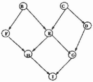
Example 3.6 Con,ider the network in F igure 3. A.uume we we the ordering (B, C, D, E, F, G, H, I) to which we apply both algorithm elim-mpe and it! 6imple6t approrimation where m = 1 and i = n. Ini­ tially the bucket of each variable will have at mod one conditional probability: bucket{!) = P(I\H, G), bucleet(H) = P( H\ E, F), bucket( G) = P(G\E, D), bucleet(F) = P ( F \ B ) , bucket{E) = P(E\C, B), bucket(D) = P( D \ C ) , bucket(C) = P(C) , bucleet(B} = P(B). Proce66ing the buckeb from top to bottom by elim-mpe generate6 functiom that we denote by h function,: buclcet(I) = P(I\H, G) bucket(H) = P (H\ E , F), h1(H, G) bucleet(G) = P(GIE,D),hH(E,F,G) bucket(F) = P(F\B), hG(E, F, D) bucket(E) = P(E\C, B), hF(E, B, D) bucket(D) = P(D\C),hE(C,B,D) bucket{C) = P(C), hn(C, B) bucleet{B) = P(B),hc(B) Where h1(H,G) = mazrP(I\H,G), hH(E,F,G) =

maznP(H[E, F) · h1(H, G), and &o on. In bucket( B) obtain the mpe value mazBP(B). hc(B), and then can generate the mpe tuple while going for­ ward. If we proceu by approx-mpe ( n,l ) in6tead, we get (we denote by 'Y the function& computed by appro:z:..elim{n, 1} that differ from tho6e generated by elim-mpe): bucket(!) = P(IIH, G) bucleet(H} = P(H\E, F), h1(H, G) bucket{G} = P (G [ E , D ), "f H ( G ) bucket{ F) = P(F[B), 'YH (E, F), bucket{E) = P(E\C,B),y(E),-yG (E,D) bucleet{D) = P(D\C),"fE(D) bucket{C) = P(C),-yE(C,B),'YD(C) bucket(B) = P(B),-yc(B),"fF(B) .

Algorithm& elim-mpe and approx-mpe ( n,l ) fir6t dif­ fer in their processing of bucket( G). There, in6tead of recording a function on three variable6, hH(E, F, G), iu6t like elim-mpe, appro:z:..mpe(n,l) record6 two function6, one on G alone and one on E and F. Once approz-mpe{n,l} ha6 proceued all bucket!, we can generate a tuple in a greedy fa6h­ ion a6 in elim-mpe: we choo6e the value of B tiWJt marimize6 the product of function6 in B 's bucket, then a value of C marimizing the product-function6 in bucket(C}, and so on.

There is no guarantee on the quality of the tuple we generate. Nevertheless, we can bound the error of appro:z:-mpe by evaluating the probability of the generated tuple against the derived upper bound, since the tuple generated provides a lower bound on the mpe.

Alternatively, we can use the recorded bound in each bucket as heuristics in subsequent search. Since the functions computed by approz-mpe{i, m} are al­ ways upper bounds of the exact quantities, they can be viewed as over-estimating heuristic func­ tions in a maximization problem. We can associate with each partial assignment ip-1 = {z1, ... , :l:p-t ) an evaluation function f(i,_l) = (g · h)(z,_1) where g(ip-1) = rrr.:� P(zi\Zpo.) and h(ip-1) = IT;ebuclcetp_1h;. It is easy to see that the evaluation function f provides an upper bound on the mpe re­ stricted to the assignment i,_1· Consequently, we can conduct a best first search using this heuristic evaluation function. From the theory of best first search we know that (1) when the algorithm ter­ minates with a complete assignment, it has found an optimal solution; (2) the sequence of evaluation functions of expanded nodes are non-increasing; (3) as the heuristic function becomes more accurate, fewer nodes will be expanded; and (4) if we use the

full bucket-elimination algorithm, best first search will become a greedy and complete algorithm for the mpe task [10].

3.1 Cases of completeness

Clearly, approz-mpe(n, n) is identical to elim-mpe because a full bucket is always a refinement-maximal (n, n)-partitioning. There are additional cases for i and m where the two algorithms coincide, and in such cases approz-mpe(i, m } is complete. One case is when the ordering d used by the algorithm has induced width less than i. Formally,

Theorem 3. 7 Algorithm appro:z:.mpe(i, n} i! com­ plete for ordered network! having w· (d) � i.

Another interesting case is when m = 1. Algo­ rithm approz-mpe(n, 1) under some minor modifica­ tions and if applied to a poly-tree along some legal orderings coincides with Pearl's poly-tree algorithm [11]. A legal ordering of a poly-tree is one in which observed variables appear last in the ordering and otherwise, each child node appears before its par­ ents, and all the parents of the same family are con­ secutive. Algorithm approz-mpe{n, 1} will solve the mpe task on poly-trees with a legal variable­ ordering in time and space O(ezp(IFI)), where IFI is the cardinality of the maximum family size. In other words, it is complete for poly-trees and, like Pearl's algorithm, it is tractable. Note, however, that Pearl's algorithm records only unary functions on a single variable, while ours records intermediate results whose arity is at most the size of the fam­ ily. To restrict space needs, we modify elim-mpe and approz-mpe{i, m } as follows. Whenever the al­ gorithm reaches a set of consecutive buckets from the same family, all such buckets are combined into one !uper-bucket indexed by a.ll the constituent buckets' variables. In summary,

Prop o s ition 3.8 Algorithm approz-mpe{n,I} with the 8uper-bucket modification, applied along a legal ordering, i! complete for poly-tree! and i! identical to Pearl'! poly-tree algo'l'ithm for mpe. The modi­ fied algorithm'! complexity i! time ezponential in the family 1ize, but it require! only linear 1pace. D

4 Approximating belief updating

The algorithm for belief assessment, elim-bel, is iden­ tical to elim-mpe with one change: it uses sum­ mation rather than maximization. Given some ev id en c e e, the p r o b l e m is to assess the belief in variable X1, namely, to compute P ( :z: 1 , e) = L-z=:! ;" II �1P(:z:i, e[:z:pa.). When processing each bucket, we multiply all the bucket's matrices, At. ... , >..i> defined over subsets S1, ... , S;, and then eliminate the bucket's variable by summation [3].

In [4] we presented the mini-bucket approximation scheme for belief updating. For completeness, we summarize this scheme next. Let Ql = {Q1, ··· , Q,.} be a partitioning into mini-buckets of the func­ tions >.1, ... , >. ; in Xp 's bucket. Algorithm elim­ bel com.putes )..P: (l index the mini-buckets) )..P = Lx, II�=l >..i = l:x, III=1 lit, >..1,. Separating the processing of one mini-bucket (call it first) from the rest, we get ).P = L:x, ( ITt , >.1,) · (W==ziTt,>.t . ) , and migrating the summation into each mini-bucket yields, �, = rrr=l Lx, rr,,>..l , . This, however, amounts to computing an unnecessarily bad upper bound on P because the product IIt,>..l, for i > 1 is bounded by .L: x, II,,>.,,. Instead of bounding a function of X by 1ts sum over X, we can bound by its maximizing function, which yields �' = .L: x ,. ( (Iltl >.h) 0 rrr=2ma:z:x,.III,AI.;)· Clearly, for ev­ ery partitioning Q, )..P::; yq · In summary, an upper bound gP of )..P can be obtamed by processing one of Xp 's mini� buckets by summation, and then process­ ing the rest of Xp's mini-buckets by maximization. In addition to approximating by an upper bound, we can approximate by a lower bound by applying the min operator to each mini-bucket or by computing a mean-value approximation using the mean-value operator in each mini-bucket. Algorithm, appro:c­ bel-maz(i, m ) , that uses the maximizing elimination operator is described in [4]. In analogy to the mpe task, we can conclude that, approz-bel-ma:c(i,m} has time complexity O(m · ezp(2i)), is complete when, (1) w"(d) � i, and, (2) when m = 1 and i = n, if given a poly-tree.

5 Approximating the map

The bucket-elimination algorithm for computing the map, elim-map, presented in [3] is a combination of elim-mpe and elim-bel; some of the variables are eliminated by summation, others by maximization. Consequently, its mini-bucket approximation is com­ posed of approz-mpe{i,m} and appro:c-bel-ma:c{i,m).

Given a belief network BN = {Pt, . .. . , P,,J, a. sub­ set of hypothesis variables A :::: {A1, . .. , Ar.}, and some evidence e, the problem is to find an assign­ m ent to the hypothesized variable that maximizes

their probability. Formally, we wish to compute

when :z: = (a1, ... , a�o, :Z:Jo+l· ... , :Z:n ) · Algorithm elim­ map, the bucket-elimination algorithm for map, as­ sumes only orderings in which the hypothesized vari­ ables appear first. The algorithm has a backward and a forward phase, but its forward phase is only relative to the hypothesized variables. The ap­ plication of the mini-bucket scheme to elim-map is a straightforward extension of approz-mpe(i,m} and approz-bel-maz(i, m}. We partition each bucket into mini-buckets as before. If the bucket's variable is a summation variable, we apply the rule we have in appro:c-bel-maz(i,m}, that is, one mini-bucket is approximated by summation and the rest by maxi­ mization. When the algorithm reaches the buckets with hypothesized variables, their processing is iden­ tical to that of approz-mpe(i,m). Algorithm approz­ map(i,m} is described in Figure 4.

Theorem 5.1 Algorithm approz-map(i, m} com­ pute"' an upper bound of the map, in time 0( e:cp( m · e:cp(2i})) and &pace O(e:cp(m · ezp(i))). Algorithm approx-map(i, n} i.! complete when w * (d) :S i, and algorithm approx-map(n, 1} u complete for poly­ tree&. D

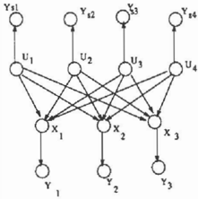
Consider a belief network appropriate for decoding a multiple turbo-code, that has M code fragments (see Figure 5, which is taken from Figure 9 in [2]). In this example, the Ufs are the information bits, the X;'s are the code fragments, and the Yi's and Y,,'s are the output of the channel. The task is to assess the most likely values for the U's given the observed Y's. Here, the X's are summation variables, while the U's are maximization variables. After the ob­ servation's buckets are processed, (lower case char­ acters denoted observed variables) we process the first three buckets by summation and the rest by maximization using appro:c-map(n, 1 } , we get that all mini-buckets are full buckets due to subsurnp­ tion. The resulting buckets are:

bucket(X1) = P(y1IX1), P(X1IUt, U:z:, U3, U4) bucket(X2) P(y:z:IX2), P (X2IUt, U2, U3, U4) f3x1 (Ut, U:z:, U3, U4) bucket(X3) P(y3IX2), P(X2IU11 U2, U3), /3 x 2 (Ull U2, U3, U4) bucket(Ut) = P ( U t ) , P(y,11Ut), f3 x · (U11 U2, U3, U4) bucket(U:z:) = P(U2), P (y ,. IU2 ), {3u1 (U2, U3, U4) bucket(U3) = P(U3), P(y,, IU3), {3 u2 (U3, U 4 ) bucket(U4) = P(U4), P(y,� IU4), f3 u · (U4) , Therefore, approz-map(n, 1} coincides with elim­ map for this network.

Algorithm approx-map(i,m) Input: A belief network BN = {Pt, ... ,P,.}; a sub­ set of variables A = {At1 ··· ,A�o}; an ordering of the variables, d, in which the A's are first in the ordering; evidence e. Output: An upper bound maximum a posteriori hy­ pothesis, A = a. 1. Initialize: Partition BN into bucket1, ·· · , bucket,., where bucket, contains all matrices whose highest vari­ able is X,. 2. Backward: For p <f- n downto 1, do for all the matrices f' t , f:J l , ... ,{3; in bucketp, do · (bucket with observed variable) if bucketp contains the observation Xp = zp1 then assign Xp = Xp to each {3; and put each resulting function into its appropriate bucket. · else, if Xp is not in A, for {3111 ··· 1{3; in bucketp1 do generate an ( i, m )-partitiorung q ' of the matrices fl· into miru-buckets Q,, ... 1 Qr. (processing first bucket) For Q1 first in q ' containing f3 t17 ···� f' t ; 1 do · generate function {3 1 = L: x ,. II 1 =1 {31 , . Add {:J1 to the bucket of the largest-index variable in U1 <f­ U1=l St, -{Xp}· I · For ea � Qr 1 l > 1 in Q contairung f3·1, ··· 1f3r; 1 do Ur � U�=l Sr, {Xp}· Generate the functions {:J1 = maxx,. nf=1{:J,,. Add {3 1 to the bucket of the largest­ index variable in U,. · else, if Xp E A, for f3t,f3l, ... 1{3j in bucketp1 do generate an ( i, m )-miru-bucket-partitiorung q ' = { Q t , ... 1Qr}· For each Q, E q ' contairung f:J111 ··· ,{:Jr., do generate function {:J11 {:J1 = maxx,.m=1{:Jr,. Add {3 1 to the bucket of the largest-index variable in U, � U1= s,, -{Xp}· 3. �orward: Assign values, in the ordering d = At, ... , A1o using the information recorded in each bucket.

Figure 4: Algorithm approz-map-maz(i,m)

6 Experimental evaluation

Our preliminary empirical evaluation is focused on the trade-off between accuracy and efficiency of the approximation algorithms for the mpe task. We wish to understand 1. the sensitivity of the approxima­ tions to the parameters i and m, 2. The effective­ ness of the approximations on sparse networks vs dense networks, and on uniform probability tables vs. structured ones (e.g., noisy-ORs), and 3, the extent to which a practitioner can tailor the approx­ imation level to his own application.

We focused on two extreme schemes of approz­ m pe {i , m ) : the first one, called approz:-mpe{m), as­ sumes unbounded i and varying m, while the sec­ ond one, called approz:-mpe{i}, assumes unbounded m and varying i.

Given the values of i and m, many (i, m)­ partitionings are feasible, and preferring a particu­ lar one may have a significant impact on the quality of the result. Instead of trying to optimize parti­ tioning, we settled on a simple strategy. We first created a canonical partitioning in which subsumed functions are combined into mini-buckets. Then, appro:rJ-mpe{m) combines each m successive mini­ buckets into one mini-bucket, while approz-mpe{i) generates an i.-partitioning by processing the canoni­ cal mini-bucket list sequentially, merging the current mini-bucket with a previous one provided that the resulting number of variables in the resulting mini­ bucket does not exceed i.

The algorithms were evaluated on belief networks generated randomly. The random acyclic-graph gen­ erator, takes as an input the number of nodes, n, and the number of edges, e, and randomly gener­ ates e directed edges, ensuring no cycles, no parallel edges, and no self-loops. Once the graph is available, for each node :z:;, a conditional probability function P(z·l:z:,.,..) is generated. For uniform random net­ works the tables were created by selecting a random number between 0 and 1 for each combination of val­ ues of :z:, and :z:,.,.,, and then normalizing. For ran­ dom noisy- OR networks the conditional probability functions were generated as noisy-OR gates by se­ lecting a random probability q1c for each "inhibitor".

Algorithm approz-mpe(i,m) computes an upper bound and a lower bound on the mpe. The latter is provided by the probability of the generated tuple. For each problem instance, we computed the mpe by elim-mpe, the upper bound and the lower bound by the approximation (either approx-mpe{m} or approx­ m p e ( i }) , and the running time ofthe algorithms. For diagnosis purposes, we also recorded the maximum family size in the input network, F;,, and the max­ imum arity of the recorded functions, F0· We also report the maximum number of mini-buckets that occurred in any bucket during processing (mb).

6.1 Results

We report on four sets of uniform random networks (we had experimented with more sets and observed similar behavior): a. set of 200 hundred instances having 30 nodes and 80 edges (set 1), a set of 200 instances having 60 nodes and 90 edges (set 2), a set of 100 instances having 100 nodes and 130 edges (set 3) and a set of 100 instances having 100 nodes and 200 edges (set 4). The first and the forth sets represent dense networks while the second and the third represent sparse networks. For noisy-OR net­ works we experimented with three sets having 30 nodes and 100 edges; set 5 has 90 instances and uses one evidence, set 6 has 140 instances and uses three evidence nodes and set 7 has 130 instances and uses ten evidence nodes.

6.1.1 Uniform random networks

On the relatively small networks (sets 1 and 2) we applied elim-mpe and compared its performance with the approximations. The results on these two sets appear in Tables 1-3. Table 1 reports averages, where the first column depicts m or i. Rather than displaying the mpe, the lower bound, and the upper bound (often, these values are very small, of order 10-6 and less), we report ratios which capture the accuracy of the approximation. Thus, the second column displays Ml1, the ratio between the value of an mpe tuple (Ma:z:) and the lower bound (Lower); the third column shows the U IM ratio between the upper bound (Upper) and Ma:z:; and the fourth col­ umn contains the time ratio, T R between the CPU running times for elim-mpe and appro:rJ-mpe(m) or approx-mpe(i). The next column gives the CPU time, T,., of appro:rJ-mpe(m) or approz:-mpe(i). Fi­ nally, F,, F 0 and mb, are reported.

Table 2 gives an alternative summary for the same two sets, focusing on appro�-mpe{m} only. Three statistics MIL, U I M ratios, vs. the Time Ratio, are reported. For each bound and for each m, we display the percent of instances (out of total 200) on which the corresponding ratio (MI1 for the lower bound, U IM for the upper bound) belongs to the interval [E- 1, E] where the threshold value, E, changes from 1 to 4. We also display the corresponding mean T R. For example, from Table 2's first few lines we see

that 8.5 % instances out of the 200 were solved by appro:tJ-mpe(m=1} with accuracy factor of 2 or less, 48% achieved this accuracy with m = 2. The speed­ up over m = 1 instances was 176 while the speed-up for m= 2 was 20.8.

Table 1: elim-mpe vs. appro:tJ-mpe(i,m) on 200 in­ stances of random networks with 30 nodes, 80 edges, and with 60 nodes, 90 edges

Mean value• on 200 _Ln•tance•
•lim-mp• v•· 4ppNe-mpt(m form- 1,�.3
m	MJL	UJM	TR	T ,.	ma>: mb	max "'•	max P.
I I I I 80 nod••· ao •da•• I I
1	43.2	41.2	211 8.1	0.1	4	9	n
2	t.O	3.3	25.0	2.2	2	�	n
3	1.3	1.1	1.t	21.4	1	9	n
I eo nod••· 90 •dsu 1 I I
1	9.9	21. '1'	131.5	0.1	3	5	12
2	1.a	2.a	27.9	0.1	2	5	n
3	1.0	1.1	1.3	11.9	1	5	12
elim-m.pe V•• CpprOit-fi'I,J'8 ,; for 1 - 3 1 t5 1 II 1:1
i	MfL	UfM	TR	T	':.�	max P,	ma>: P.
I ., I !0 node11 AO edae•1 � ...-aluel per node
3	55.5	41.4	309.2	0.1	4	9	12
I	29.2	20,'1'	254.8	0.1	3	9	12
II	1'1'.3	'1'.5	1111.0	0.2	3	9	12
12	15.0	3.0	U.3	0.8	2	9	12
I I 80 node11 90 ed 1 e11 � Yalue• per node 1
3	1.1	18.5	138.2	0.1	3	5	12
I	2.8	8.1	112.8	0.1	2	5	12
II	1.9	2.1	'11.'1	0.2	2	5	12
12	1.4	1.8	24.2	0.5	2	5	12

I

From these runs we observe a considerable efficiency gain (2-3 orders of magnitude) relative to elim-mpe for 50% of the probelm instances for which the ac­ curacy factor obtained was bounded by 4. We also observe that, as expected, sparser networks require lower levels of approximations than those required by dense networks, in order to get similar levels of accuracy. In particular, the performance of appro:tJ­ mpe(i=a) gave a 1-2 orders of magnitude perfor­ mance speedup while accompanied with an accuracy factor bounde by 4, to 80 percent of the instances on dense networks, and to 97 percent of the sparse net­ works. From table 1 we also observe that controlling the approximation by i provides a better handle on accuracy vs efficiency tradeoff. Finally, we observe that approz-mpe(m=l} can be quite bad for arbi­ trary networks.

We experimented next with larger networks (sets 3 and 4), on which running the complete elimina­ tion algorithm was sometimes computationally pro­ hibitive. The results are reported in Tables 4 and 5. Since we did not run the complete algorithm on those networks, we report the ratio U /L. We see that the approximation is still effective (a factor of accu­ racy bounded by 10 achieved very effectively) for sparse networks (set 3). However, on set 4, appro:tJ-

Table 2: Summary of the results: M/L, U /M and TR statistics for the algorithm approz -mpe(m) with m = 1, 2, 3 on random networks

Random network• w1th 30 nodes, 10 edc••
[� -l,�J	m	Lower bound		Upper bound
		MfL	Moan TK	UfM	Mean TR
��·�l	1	1.5!'	1'1'8.4.	0!'	o.o
[2,3]	1	9.0%	339.11	o%	o.o
[3,4]	1	1.6%	221.3	0%	0.0
[i, oO]	1	'14%	313.1	100%	291.1
��·�l	2	tU'o	20.1	211.5,..	10.11
[2,3]	2	11%	211.'1'	2'1.11%	22.2
\ 3,	2	'1'.6%	113.1	17%	22.1
r ·�� ..	2	211.5%	25.3	21%	41.0
"" l 1 · �!	3	92,..	1.4	9'1'7i	1.4
[2,3]	3	5%	2.0	3%	4.9
(3,4}	3	1%	1 .2	1%	1.3
[ t, oO]	3	3%	1.1	0"'	o.o
Random notworko W1th eo nodoo, 90 •da••
L• 1, •J	m	Lower bound		Upper bound
		MfL	M ... uTR	UfM	M ... uTR
!�· �l	1	26.11:'-	1'1'2.8	o,.,	o.o
(2, 3]	1	18%	84.3	oYo	o.o
	1	9Yo	43.5	!Yo	17.4
r!M � l 4., 00	1	U.IIY,	H7.5	119%	132.'1'
!�· �!	2	'1'9.5,..	:1 1 . 1	41�	:11.2
[2, 3]	2	10%	:11.0	31%	!:I.e
\3, " l	2	6.5%	-!:1.4	14%	24.t
r � 4,""	2	15%	40.5	U%	40.3
!�· �!	3	1ooy;	1.3	100yj	1.3
[:1, 3]	3	o%	1.0	1Yo	1.0
[3,t]	3	o%	0.0	oYo	0.0
4	3	0%	0.0	OYo	0.0

[ 4 , oO]

mpe(m} was too expensive to run for m = 3, 4, and too inaccurate for m = 1, 2. For this difficult class, an acceptable accuracy was not obtained.

6.1.2 Noisy-OR networks

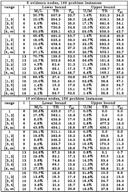
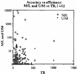
We experimented with several sets of random noisy­ OR networks and we report on three sets with 30 variables and 100 edges. The results are summa­ rized in Figure 6 and Table 6. In the first, we display all instances of set 5 plating the accuracy (M/L and U /M) vs T R, for all 90 instances. In the second we display the results on sets 6 and 7 in a manner similar to Table 2. T.,1 gives the time of elim-mpe.

The results for the noisy-OR networks are much more impressive than for the uniform random net­ works. The approximation algorithms often get a correct mpe while still accompanied by 1-2 orders of magnitue of speed-up (see cases when i = 12 and i = 15.) Although the mean values of U /M and M/1 can be large on average due to rare instances (see Figure 6), in many of the cases both ratios are close or equal to 1.

In summary, for random uniform and noisy-OR net­ works, 1. we observe that very efficient approxi­ mation algorithms can obtain good accuracy for a considerable number of instances, 2. appro:tJ-mpe(i) allows a more gradual control of the accuracy vs. ef-

Table 3: Summary of the results: M/L, U /M and TR statistics for the algorithm a ppr ox -mpe( i) with i = 3, 6, 9, 12 on random networks

Random net.... orkl Wlth 30 nodelt eo edge•
[• 1 , • l	I	Lower bound		Upper bound
		MfJ..	Mean :R	UfM	Me•n :R
· ��	6	111.5, ,	210.1	o.s, ,	11.3
� � [2, 3]	6	9%	266.6	o%	0.0
[3, 4]	6	6.5%	2-18.7	0.&%	14.4
[4, oo]	3	69%	250.1	99%	256.11
!1• 2 !	9	31!'i	150.1	2.6'r o	33.0
[2, 3)	9	10%	100.5	7%	101.1
(3 , 4)	9	10.5%	114.7	12.6%	132.9
[ !, ..;]	9	41.6%	169.8	78%	162.1
	n	61 !'!	41.3	29!'i	27.0
!�· �! [ 2, 3]	n	15%	41.3	32%	60.5
�3, 4�	12	11%	69.2	IT%	U.4
[ 1 4, 00	6	23%	u.s	22%	60.6
Random network• •ith 60 node11 SID edgea
! • 1, • J	I	Lower bound		Upp e r bound
		MfJ..	M.ean .....,.	UfM.	mean .....,.
�	6	&1.�:' ·	91.4	3, .	2&.&
��· � [2, 3]	6	15%	1511.3	15.5%	71.0
[3 , 4]	6	9%	U.3	17.!i%	57.2
�	6	1&.5%	157.2	64%	U2.0
r: ·.�	9	ao, ,	54.9	3S.&!'i	35.9
��· �� [2, 3]	9	11.5%	88.9	2&%	72.0
[3 , 4]	9	3%	27.4	21"	96.3
[4 , oo)	9	5.5%	158.-!	u.s%	124.5
��· ��	12	au;:' !	2-!.4	II,.	23.5
[2, 3]	12	u.s%	29.7	13.&%	29.1
(3, -!J	12	0.5%	1 1.4	&%	37.3
[4 , oo]	12	2.&%	21.1	0.5%	H.O

ficiency tradeoff than approx-mpe(m); 3. on random noisy-OR networks appro:c-mpe(i} obtains a good ap­ proximation ( M/L < 1.5) while still improving ef­ ficiency relative to the complete elimination by one or two orders of magnitude.

7 Conclusions and related work

The paper describes a collection of parameterized algorithms that approximate bucket elimination al­ gorithms. Due to the generality of the bucket-

Table 4: elim-mpe vs. appro:c-mpe(i,m) on 100 in­ stances of random networks with 100 nodes and 130 edges

Mean vala•• on 100 l �•tan.aea tdim-m.pe v•. e&ppr-'rt:.-mp � m j_
m	UfL	T•	mn mb	max .!1' .;
1	7111.1	0.1	3	5
2	10.t	3.4	�	5
3	1.2	13�.5	1	6
4	1.0	209.5	1	5
elim.-m.pa v•. 4ppPoc-mpe i
i	UfL	T..	max mb	max .!1' .;
3	''T&.S	0.1	3	5
6	36.3	0.2	2	5
I	14.5	0.3	l	5
12	1.1	o.s	2	&
u	3.0	3.7	l	5
11!	l.T	H.ll	1	5

Table 5: elim-mpe vs. approz-mpe{i) for i = 3 - 21 on 100 instances of random networks with 100 nodes and 200 edges

Mean vlllne• on 100			ln•tance•
'	UfL	T.,	max mb	max
3	1350t27.6	0.�	"	Pi 7
6	234561.7	0.3	3	T
9	9064,4	0.&	3	'T
12	2 5 U .9	1.8	3	7
1&	7]{.1	10.6	3	7
18	•o1.a	75.3	3	1
2 1	99.6	5&0.2	2	1

elimination framework, both the parameterized al­ gorithms and their approximations will apply uni­ formly across many areas. We presented and ana­ lyzed the approximation algorithms in the context of several probabilistic tasks. We identified regions of completeness and provided preliminary empirical evaluations on randomly generated networks.

Our empirical evaluations have interesting negative and positive results. On the negative side, we see that when the approximation algorithm coincides with Pearl's poly-tree propagation algorithm (i.e., when we use approz-mpe(m=l}), it can produce ar­ bitrarily bad results, which contrasts recent suc­ cesses with Pearl's poly-tree algorithm when ap­ plied to examples coming from coding problems [2; 9]. On the positive side, we see that on many prob­ lem instances the approximations can be quite good. As theory dictates, we observe substantial improve­ ments in approximation quality as we increase the parameters (m or i). This allows the user to an­ alyze in advance, based on memory considerations and given the problem's graph, what would be the best m and i he can effort to use. In addition, the ac-

3 e.,.tdenee node11 lofO problem 1nd•nce1
ranae	I	Lower bound			Upper bound
		M,IL rR			UfM	rR	T,l
1	5	20.79 �	&07.9	r,, 22.7	1.4 '!	&21.2	24.3
[1 , 2]	6	10.0%	6&4.2	21.0	16.4%	616.1	21.2
[2, 3]	6	&.0%	494.1	2&.&	17.1%	611.6	34.1
[3, 4]	5	4.3%	730.&	34.1	10.0%	421.&	11.1
[,, .,.;]	6	60.0%	929.1	43.2	&&.0%	939.0	i].7
1	9	46.4"	461.0	33.7	1.4'!	&10.1	40.9
[1 , 2]	9	1&.0%	&23.2	39.0	40.7%	319.4	21.\1
(2, 3]	9	10.0%	431.4	34.3	22.1"	&12.3	n.2
(3, 4]	9	1.4%	411.1	27.2	1&.0%	730.&	&&.&
[i, .,.;]	9	27.1 Yo	&3&.3	40.0	20.7%	402.1	30.7
1	12	70.7Y,	129.0	32.0	u.sy,	11&.5	25.1
[ 1 , 2]	12	10.7%	202.6	&0.1	&6.4%	1&1.1	u.s
[2, 3]	12	4.3%	12.4	21.2	11.<1%	11&.3	31.6
[3, i]	1:1	2.9%	69.1	17.2	7.1%	1111.7	u.s
.,.;]	1:1	11.4%	224.2	58.7	6.4%	149.1	37.&
[,, 1	1&	16.4,. ,	:n.t	34.1	40.7%	11.7	22.2
[1 , 2]	1&	10.0%	36.0	4&.0	&2.9%	38.8	47.1
[2, 3]	1&	1.4%	13.2	17.9	&.0%	28.0	34.7
[3, 4]	1&	0.7%	9.0	13.1	0.7%	11.11	17.1
[,, .,.;]	1&	2.1"	u.r	62.5	1.4%	35.6	31.5
10 e·ndence node•, 130 problem Lnltanc:e•
ran1e	i	Lower bound			Up er bound
		MfL	'.1:11.	"l"ol	UfM	TK	:t"ol
1	I	28.5!!	423.0	17.1	0.0�	0.0	0.0
[1, 2]	8	17.3%	312.1	15.1	0.0%	0.0	0.0
[2, 3]	I	6.0%	43!.9	17.4	2.3%	204.1	11.:1
[3, i]	I	6.8%	436.0	11.3	0.1%	t17.2	19.0
[i, .,.; ]	6	43.8%	454.1	19.8	97.0%	436.1	11.1
1	9	39.1'Jio	311.1	19.4	O.O'Jio	o.o	o.o
[1 , 2]	9	19.&%	212.8	19.2	3.8%	90.&	&.3
[2 , 3]	9	9.1%	2U.2	14.5	6.0%	206.6	13.&
(3, i]	9	6.0%	222.7	14.2	10.&%	170.3	11.3
[,, .,.;]	9	2&.8%	260.&	18.1	79.7%	310.0	19.7
1	12	&4.9!!	87.2	18.8	0.1'!	&.1	0.7
[1 , 2]	n	19.&%	82.1	17.2	21.1%	80.3	12.&
[ 2, 3)	12	3.8%	74.1	15.4	14.3%	92.4	18.4
[3, 4]	12	4.&%	111.1	13.1	11.3%	57.6	12.1
[4 , oo]	12	17.3%	12.9	11.1	51.9%	91.1	21.8
1	1&	73.7'Jio	18.6	11.9	ll.l,..	10.3	II.&
[1, 2]	1&	12.1%	18.3	17.4	34.1%	14.3	13.0
			18.1	22.2	18.&%	24.7	24.4
[2 , 3] [3 , 4)	15 1&	3.0% 3.1%	21.4	15.7	1.3%	19.&	11.4
[4, oo)	15	7,&%	31.11	25.1	19.5%	27.8	29.1

curacy of the result can be evaluated by comparing the lower and upper bounds generated. The poten­ tial of this approach for heuristic guidance in search, still needs to be tested.

The mini-bucket approximations parallel consis­ tency enforcing algorithms for constraint pro­ cessing, in particular those enforcing directional consistency [5]. Specifically, algorithms such as adaptive-consistency or adaptive-relational con­ sistency are full bucket-elimination algorithms [7]. Their approximation algorithm, directional­ relational-consistency(i,m) [7], enforces bounded levels of directional consistency. In propo­ sitional satisfiability, bounded-directional-resolution with bound b corresponds to the mini-bucket algo­ rithm with i = b [6 ] . Recently, a collection of approx­ imation algorithms for sigmoid belief networks was presented in the context of a recursive algorithm sim­ ilar to bucket elimination [8] . It is shown [8] that an upper and lower bounds approximations can be de­ rived for sigmoid belief networks. Specifically, each Sigmoid function in a bucket, is approximated by a Gaussian function.

References

1. S. A. Arnborg. Efficient algorithms for combinato­ rial problems on graphs with bowtded decompos­ ability a sw-vey. BIT, 25:2-23, 1985.
2. R. McEliece D. C. MacKay and J. Cheng. Turbo decoding as an instance of pearl's "belief propaga­ tion" algorithm. 1996.
3. R. Dechter. Bucket elimination: A unifying f rame­ work for probabilistic inference algorithms. In Un­ certainty in AI (UAI-96), pages 211-219, 1996.
4. R. Dechter. Mini-buckets: A general scheme of gen­ erating approximations in automated reasoning. In International Joint Conference on Artificial Intelli­ gence (IJCAI-97 ), 1997.
5. R. Dechter and J. Pearl. Network-based heuristics for constraint satisfaction problems. Artificial In­ telligence, 34:1-38, 1987.
6. R. Dechter and I. Rish. Directional resolution: The davis-putnam procedure, revisited. In Proceeding· of Knowledge Repre1entation (KR-94}1 pages 1341451 Bonn, Germany, 1994.
7. R. Dechter and P. van Beek. Local and global re­ lational consistency. Theoretical Computer Science, pages 283-308, 1997.
8. T. S. Jaakkola and M. I. Jordan. Recursive algo­ rithms for approximating probabilities in graphical models. Advance· in Neural Information Proceuing Sy1tem1, 9, 1996.
9. F. R. Kschlschang and B.H. Frey. Iterative decoding of compound codes by probability propagation in graphical models. 1ubmitted, 1996.
10. J. Pearl. Heuristics: Intelligent search strategies. In Addi1on- We1ley, 1984.
11. J. Pearl. Probabilistic reasoning in intelligent sys­ tems. In Morgan Kaufmann, 1988.