A Stratified Simulation Scheme for Inference In Bayesian Belief Networks

Remco R. BouckaertPhD student

Utrecht University Department of Computer Science P.O.Box 80.089 3508 TB Utrecht, The Netherlands r em c o @ cs. r uu.n l

Abstract

Simulation schemes for probabilistic infer­ ence in Bayesian belief networks offer many advantages over exact algorithms; for ex­ ample, these schemes have a linear and th us predictable runtime while exact algo­ rithms have exponential runtime. Exper­ iments have shown that likelihood weight­ ing is one of the most promising simulation schemes. In t h i s paper, we present a new simulation scheme that generates samples more evenly spread in the sample space than the likelihood weighting scheme. We show both theoretically and experimentally that the stratified scheme ou t pe r for ms likelihood weighting in average runtime and error i n estimates of b e lief s .

Keywords: Bayesian belief networks, ev­ idence propagation, simulation, stratifica­ tion.

1 Introduction

Simulation schemes [ Chavez and Cooper, 1990; Hen­ rion, 1988; Pearl, 1992; Shachter and Peot, 1990] of­ fer simple and general-purpose procedures for inex­ act p r obab ili s t ic inference in Bayesian belief n e t wo r ks . The basic idea underlying these schemes is to generate a set of samples and to approximate beliefs of various variable values by the frequency of appearance in the sample.

Exact inference in Bayesian belief networks has been proven NP-hard, [ Cooper, 1990]; so, exact algo­ rithms [Lauritzen and Spiegelhalter, 1988; Pearl, 1988; Shachter, 1988] all have an exponential in the num­ ber of variables complexity. T ho ug h when demanding a certain accuracy in beliefs, runtimes of simulation schemes are also NP-hard [Dagum and Luby, 1993] and an exponential in the number of nodes amount of s am pl e s is necessary, the runtime is linear in the number of samples and variables.

The complexity of exact methods strongly depends on the topology of the network; especially when many loops occur in a network, the performance of exact methods decreases dramatically. However, for simu­ lation schemes the topology of the network does not m at t er . In many applications exact inference may not be necessary since, due to inexactness of the proba­ bility assessments in the network, approximate beliefs suffice.

However, observation of values of v a r ia bles and prop­ agation of this evidence tends to decrease the perfor­ mance of simulation schemes; many samples may be very non-specific for the observed situation and only a small portion of the samples may influence the es­ timates of beliefs. Therefore, it is important that a s imu l at ion scheme g ener a t es a lot of samples e v e nl y distributed over the sample space. Generating such samples in an efficient way i s the topic of the present paper.

In Section 2, we review some of the most popular sim­ ulation schemes in a general framework. In Section 3, we present a new scheme based on a popular statisti­ cal technique called stratification. The complexity and several optimizations of this scheme are described. In Section 4, we present experimental results comparing various simulation schemes. We end with conclusions in Section 5.

2 Simulation Schemes for Ba y esian Belief Networks

Let U = {x1, . . . ,xn}, n?. 1, be a set of variables; for simplicity we assume the variables are d i s c r e t e . A Bayesian belief network B over U is a pair (Bs, Bp) where the network structure Bs is a directed acyclic graph with one node for each variable in U. Bp is a set of conditional p rob a b i l i ty tables. For every variable Xi E U, the s e t Bp contains a conditional probability table P(xil11'i) that enumerates the probabilities of all values of Xi given values of the variables in its parent­ set 1ri in the network structure Bs. The probability dis t r i b u ti o n represented by such a belief network B is TI,,EU P(xil11'i), [P ea r l , 1988].

Let E be the set of values of observed variables. In­ ference in a belief networks amounts to calculating the beliefs Bel(x) in each variable x, that is the proba­ bility of the values of each variable given E, P(xiE). Simulation schemes aim to approximate these beliefs by randomly generating samples. A sample is a value assignment to all variables in U, also called instantia­ tion. The scheme keeps track of the relative frequency of variable values in the samples called the score.

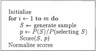
In Figure 1, a general sampling algorithm is depicted which we will use as a general framework to de­ scribe various simulation algorithms. Depending on the method of sample generation, an initialization pro­ cedure is executed. Then, m samples are generated and for each generated sample 5, the quotients of the probability of the instantiation, P ( 5 ) , and the proba­ bility of generating the instantiation, ?(selecting 5), is calculated. With this value, the score is updated. Eventually, the scores are normalized to obtain the beliefs.

First, we concentrate on methods for generating sam­ ples and initialization, and turn to scoring methods shortly. Henrion [Henrion, 1988] introduced a sam­ pling algorithm for belief networks. The value assign­ ments of the separate variables are chosen equiproba­ ble; the probability of selecting an instantiation there­ fore is equal for all instantiations. No initialization is performed for this scheme. A slight optimization is to generate only values for the variables for which no evi­ dence has been obtained. These variables get assigned their observed value in each sample. The value of p is calculated by I1x,EU\E P(x;l7r;). We call this scheme the simple scheme.

Another method of sample generation was proposed in [Henrion, 1988]. First, values for the root nodes of the network are generated with probabilities equal to the probabilities of the probability table first. Then, for the nodes of which all parents have been assigned a value values are generated with probabilities equal to the chance of these nodes given the values assigned to their parents. For this procedure it is handy to have a topological ordering on the variables which needs to be calculated during initialization. Again, evidence nodes are assigned their observed values in each sample. The value of p is calculated by IIx,EE P(x;l7r;). We call this method likelihood weighting. This method is also known as logic sampling [Henrion, 1988] and evidence weighting [Fung and Chang, 1990; Shachter and Peot, 1990].

The last method considered here was proposed by Pearl [Pearl, 1992] which relies on Markov blankets. The Markov blanket Bl(x;) of a node Xi consists of the parent-set of x;, the children of x; and the parents of these children except for Xi itself. In this method, a sample is not generated independent of the previous samples. When generating a new sample the previ­ ous sample is taken into account: the new value of a node x is chosen with probability proportional to the

_

product of probabilities in its Markov blanket B l (x ), ITx,EBl(x) P(x;i'lfi). Note that the probability of se­ lecting a sample 5 is P(5), sop= L As in the other methods, evidence nodes are assigned their observed value. We call method procedure Pearl's scheme.

We consider two scoring methods; simple scoring and Markov blanket scoring. Simple scoring is done by adding the value p yielded by the sample generating method for a sample S to the score of each variable with the value it has in 5. A more effective approach [Pearl, 1992] seems to add p to every value of the vari­ able weighted by the probability of its Markov blanket. The latter method will be called Markov blanket scor­ ing. For the simple and likelihood weighting scheme extra work needs to be done when Markov blanket scoring is used namely the calculation of the product of the probabilities over the Markov blankets. How­ ever, for Pearl's scheme these probabilities are already available, so little extra work needs to be performed for this scheme.

3 A Stratified Simulation Scheme

Stratification is a popular statistical technique for ob­ taining samples that are more uniformly spread in the sample space. A description can be found in any ba­ sic book on sampling. The basic idea is to divide the sample space into so-called strata, and choose in each stratum a given number of samples. Such samples rep­ resent the distribution better than randomly chosen samples, because it is not possible that no samples are taken from a large area of the sample space. So, less samples are required for a similar error in esti­ mates. There is a large freedom in selecting strata. In our approach, we will split the sample space into m equally likely strata an choose one sample from each stratum. As in Pearl's scheme, we allow some depen­ dence among samples. This dependence makes it pos­ sible to generate the samples faster than in the simple, the likelihood weighting and Pearl's scheme.

3.1 Stratification for Bayesian Belief Networks

Let the variables in U be ordered x1, ... , Xn. For ease of exposition, assume all variables to be binary taking values from { 0, 1}. Then, instantiations of U can be

0

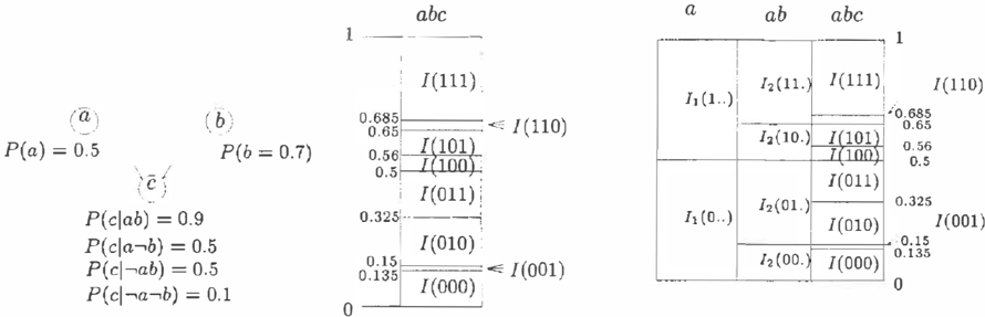
Figure 2: Belief network and corresponding intervals.

ordered according to 0 < 1 taking order of variables in account. With each instantiation S of U we associate an interval I(S) defined by,

where lo(S) = P(U < S) = LS'<S P(S'), and h i ( S ) = lo(S) + P ( S ) . The unit interval is divided into subintervals and every instantiation of U is as­ signed such a subinterval. Alternatively, every number r in the unit interval corresponds to an instantiation S of U such that r E I( S ) . For example, let U = {a, b, c} and let P(U) be defined by the Bayesian belief network depicted in Figure 2. Suppose that the variables are ordered a, b, c, we have for the values a = 0, b = 1, and c = 0, that is instantiation S = 010, the in­ terval 1(010) associated with S which is [0.15, 0.325). Since lo(S) is P(OOO) + P(001) = 0.15 and hi(S) is P(S) = 0.5 x 0.7 x 0.5 = 0.175 plus lo(S) which equals 0.325.

The stratified simulation scheme is based on using these intervals to determine samples. In its simplest form, a number r is randomly chosen from the unit interval and the instantiation corresponding to the in­ terval that includes r is the sample generated. In our example, suppose that the number r = 0.2345 is cho­ sen. Then, r is in the interval [0.15, 0.325) correspond­ ing to instantiation S = 010. So, the sample a = 0, b = 1 and, c = 0 is generated.

By imposing certain restrictions on the number cho­ sen from the unit interval, a more efficient simulation scheme is yielded. Suppose m random numbers are chosen in the unit interval and these numbers then are considered in ascending order. Now suppose that the numbers r1 = 0.2345, r2 = 0.4567, and r3 = 0.6789 have been generated. The sample corresponding to the first number is sl = 010, to the second s2 = 011, and to the third 53 = llO. Observe that for the samples S1 and S2 only the least significant bit has changed. In general, when the random numbers are considered in ascending order, then only the k least significant bits change and the nk most significant bits do not. This

a

property can be exploited to get a more efficient sim­ ulation scheme. We only have to put computational effort in assigning values to these least significant vari­ ables, while in the other simulations schemes, all vari­ ables need to be updated. However, we need to do some extra work to determine which variables need to be updated. To do so, we generalize the definition of intervals to apply to prefixes of instantiations.

Let pref�c(S), 0 :-::; k :-::; n, be the prefix of k bits of in­ stantiationS. So, preh(0111) is 011 and prefi(0111) is 0. Then, the intervals generalized to prefixes h(S) associated with instantiation S is defined by,

where lo�c(S) P(pref�c(S' ) < prejk( S )) = 'Lprefk(S')<preh(S) P(S') and h i�c ( S ) = lo�c(S) + P(prefk(S') = prefk(S)) = Lpreh(S')�prefk(S) P(S'). Note that for k = n we have the original definition for intervals, that is h( S) = I(S), and fork= 0, we have the entire unit in­ terval, I0(S) = [0, 1). Figure 3 shows the intervals for our example; h(Ol.) starts at 0.15 since P(preh(S) < 01) = P (OOO ) + ?(001) = 0.15 and ends at 0.5 since P(pref2(S) = 01) = P( 010) + P(Oll) = 0.35. Also from this definition follows that h(S) � h-t (S).

Therefore, when we are looking for an interval that contains Ti and we the previous sample is instantiation Si-t, first we check if r; is in In(S;_t). If it is not, we check if it is in In-1(5;_1) and so forth, until we find a k such that Ti is in h(S;_I) = [lo�c(Si-l),hi�c(S;_I)). Now observe that for all j, loj(Si-d is smaller than r;. So, only hij(S1_I) need to be considered; looking for k such that hi�c(S;_I) > r and hik+l < r is suffi­ cient. Since hik(S1_t) is a descending function of k, this procedure can be performed with binary search, which costs at most logn operations ( all logarithms in this paper are to base 2 unless stated otherwise). Note that this procedure easily generalizes to non-binary variables.

However, we will not generate numbers randomly in the unit interval and then consider them in ascend­ ing order. Instead, we divide the interval into m equal

lo +-0; ho +-1 for i + -1 to n do li +-0 if x; E E then val; +- e i hi +- hi-1 else val; +-0 hi +- hi-1 * P, (o)

strata where m is the number of required samples, and for each stratum we generate one random number Ti­ This procedure guarantees that the samples are uni­ formly chosen from the sample space.

3.2 An Algorithms for the Stratified Scheme

Based on these observations we formulate a stratified scheme for generating samples that fits in the general algorithm shown in Figure 1 of the previous section. The strata are regarded in ascending order. In each stratum a number r is randomly chosen. For that stratum, dynamically a new instantiation and new in­ tervals are calculated. We need to define initialization and sample generation methods. In Figure 4 and 5, pseudo-code for these methods is shown. The values of the variables for a sample is stored in the array val. We keep track of the intervals in the arrays l and h for respectively the lower and upper bound of the intervals of the instantiation stored in val. For initialization, an instantiation 50 is generated in which the value of each variable is set to 0 except when there is evidence for the variable. Obviously, the lower bounds of the in­ tervals are 0 initially, that is loJ(So) = 0, 0 � j � n. The upper-bound hij(S0) is the upper-bound of the previous interval hj_l(S0) times the probability P i(O) of choosing the value of variable XiThere are several ways of defining P. When P i is chosen the reciproce of number of values Xi can take, all states are equiproba­ ble and this scheme will be referred to as the stratified simple scheme. However, one can also take for P the probability of choosing that value of variable x; given its parent as instantiated in val. This scheme will be referred to as the stratified likelihood scheme. Note that evidence nodes do not contribute to the interval.

Figure 5 shows pseudo-code for the method for gen­ erating a sample. First, a random number r in the ith section is generated. Using binary search, the first variable Xj for which h1 < r and hj-1 > r is identi­ fied. For the variables x1 up to Xn a new value will be calculated while the values vah up to valj-l re­ main unchanged. The boundaries of the intervals of x1 are calculated from the boundaries of XJ-1; if X J is an evidence node then the boundaries are the same

f t(random[O: 1) + i1)/m j +-Binsearch (f, h) while j <= n do if Xj E E then lj +-lj1 hj +- h]-l else kt-0 l J +-lj-1 -hJ + l 1 + (hJ-1 -lJ-d * P1( k ) while f > hj do k + - k +l lj +- hj -h1 +-l J + (hJ-I -l1_I) * Pj( k ) val1 + - k jt-j+l return( val)

as for x1_1. If Xj is not an evidence node then they are bounded by the boundaries of X J -I· The value of variable x 1 is calculated by stepping through the range of Xj until the boundary encloses r.

3.3 Performance of the Stratified Scheme

Now we consider the amount of work that needs to be perf � rmed for generating m samples in a belief net­ work with n nodes. When generating a new sam­ ple, our scheme saves the work of determining values for k variables at the cost of at most log n compar­ isons. We investigate the computational complexity of our scheme in further detail. Suppose all variables are binary. Then, the most significant non-evidence variable gets assigned a value at most twice by our scheme, the second most significant non-evidence vari­ ables at most four times, etcetera; the llog m J th up to the nth. Less significant non-evidence variables all get assigned a value at most m times because they can­ not get 2 Llog mJ +k ( k > 0) times an assignment in m samples. So, at most

variable assignments are performed. At most m times a binary search is performed. Using L�=O 21c = 2x -1 and including the binary searches, we find that sample generation involves at most,

operations. We find that our scheme has a computa­ tional complexity of order O((nlog �)m). When the arity of the variables is at most k, this becomes O((n _1c log � log2 n ) m ) . Note that if the number of

samples m is larger than the number of variables, the stratified simple and likelihood weighting scheme are more efficient than the simple and likelihood weighting schemes which are of complexity O ( n.m ) .

We conclude our analysis by observing that the com­ plexity bound is conservative; if probabilities of the lower ordered variables are close to one and the strat­ ified likelihood weighting scheme is used, a much smaller number of samples is chosen for stratified schemes. It is assumed that the work for one compari­ son in a binary search is equally expensive as determin­ ing the value of a variable; however, for determining the value of a variable x, its probability table need to be looked up which may be relatively expensive if x has many parents.

In general, estimates of beliefs become more accu­ rate when the number of samples increases. Dagum and Horvitz [Dagum and Horvitz, 1993] showed that for the likelihood weighting scheme, to output a be­ lief in a value of a variable x that with probability higher than 1 -o has relative error less than t:, at least a·ln(4jo)j(t2Bel(x)) samples are required where a is the maximum value of the weighting distribution. Consider once more the example of Figure 2. For even numbers of samples, always an equal number of sam­ ples with a = 0 and with a = 1 will be generated. This results in a correct estimate of the probability of a namely P(a) = 1/2. So, the algorithm also pro­ duces better samples, a point stressed in [Chavez and Cooper, 1990] to be very important. Especially for variables that are low in the ordering good samples are produced. I feel that the bound of Dagum and Horvitz may be taken as upper bound to the number of samples to be generated.

3.4 Further Optimizations

The previous section presented a new sample scheme that is shown to be faster than other popular sampling schemes. In this section, we give attention to details of the scheme in order to get a better performance.

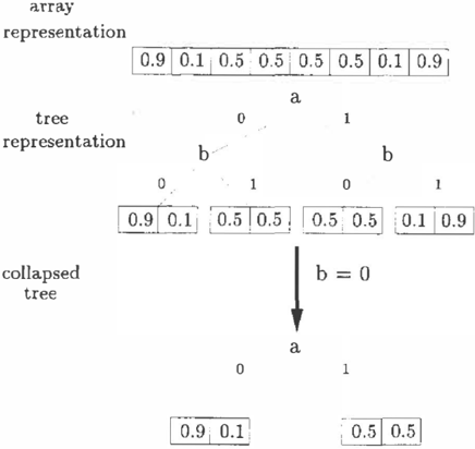
It is desirable to generate many samples in a small amount of time. To do so, it is important to choose the data-structures to be used carefully. Since condi­ tional probability tables are accessed very often, we fo­ cus on the data-structure to store these tables. These tables may be stored in an array; the basic idea is illustrated in Figure 6 for the probabilities from the tables of variable c of the example of Figure 2. For example, in CABeN [Cousins et al., 1991], a collec­ tion of algorithms for belief networks, probability ta­ bles are implemented this way. Note however that to access the array an index needs to be calculated from the instantiation of the parents of this variable. The calculation of such an index requires computationally expensive multiplications. If the network contains bi­ nary variables only however, the multiplications can be replaced by shift operations. In experiments on a HP-9000 series 700 using a C-program using shift op-

erations instead of multiplication for calculating the array index resulted in a 15% reduction of computer time.

Instead of arrays, search trees offer an alternative data structure for storing probability tables. A search tree is a tree in which on a node a choice is made which branch to take and the leafs contain information. In Figure 6 such a search tree for the probability table of the variable c from Example 6 is depicted. To find the required probability, only a pointer needs to be passed through the tree and no multiplication is per­ formed. In experiments on a HP-9000 series 700 using a C-program using search trees instead of arrays to store probability tables resulted in a 30% reduction of computer time.

The search tree also offers other advantages. When ev­ idence is observed, outgoing arcs of the observed nodes can be removed [Gaag, 1993] and the probability ta­ bles can be collapsed; the idea is that if variable x is observed to be 1 then all children of x will not use probabilities conditioned on instantiations in which x is not 1. Therefore, those probabilities can be removed from the probability table. To implement this, a search tree that stores the probability table can be pruned; only those leaves in the search tree for which the ob­ served value is present need to be stored. This is an almost trivial action for trees while it would require considerable computing for arrays. For example when b is observed to be 0, the search tree for the represen­ tation of the probability table of c can be replaced by the lower tree depicted in Figure 6.

Not only the choice of data structures is important for optimal performance. The stratified likelihood weight­ ing scheme needs a topological orde-ring on the vari­ ables. Such an ordering is not unique. To fully ex­ ploit the reduction in time achieved by the stratified

scheme, variables with high probabilities should occur foremost in the ordering; in that case they won't need a change of value too often. Therefore, when deter­ mining a topological order of the variables, their prob­ ability tables should be taken in consideration. In our experiments, we used the average probability to the power four L� 7r P(xil11'i)4 / Lx 7r 1 as an extra cri­ terion to sort t h � � ariables since i t ' a � signs extra weight to probabilities close to one; small probabilities vanish while large probabilities contribute a lot to this sum. However, we think it is worth to investigate other cri­ teria. Since when evidence is observed, outgoing arcs of the observed nodes can be removed, less constraints are left for choosing a topological ordering; children of observed nodes may be shifted lower in the ordering if their probabilities are high enough.

So far, we assumed that a random number in each section was chosen. However, also the median of the interval can be taken. At least for the lower ordered nodes, no change in estimates are expected. In fact, these estimates will become better because less errors due to random fluctuations are introduced. For vari­ ables high in the ordering however, it has the same effect as choosing a random number.

Care must taken when networks with many variables are used; the values of lok(S) and hik(S) may be er­ roneously calculated as equal due to numerical round off errors. Therefore, the representation size used for lok(S) and hik(S) need to be taken large enough. If a random number is chosen from a section, also this random number must have enough precision to avoid biases.

4 Experimental Results

We have performed some experiments to compare the stratified simulation scheme with the simple scheme, likelihood weighting and Pearl's scheme. We gener­ ated randomly ten belief networks with fifty binary variables and a poly-tree structure. The networks were generated by ordering the variables, randomly pick two nodes a and b and adding the arc a --+ b if a is lower or­ dered than b. Otherwise the arc b --+ a is added. This step is repeated but now one variable is randomly cho­ sen from the variables that are connected to at least one arc and one variable is chosen from the variables that are connected to no arc. This last step is repeated till all arcs are placed.

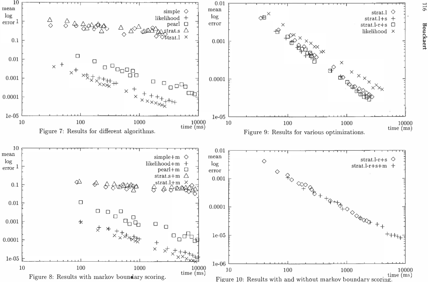
With these ten networks we applied the four algo­ rithms generating 100 up to 1000 samples, increas­ ing by 100 in each test, and further, from 1000 with steps of 1000 up to 10000 samples. So, with every network 19 different sets of samples were generated. The probability tables were stored in search trees as described in Section 3.4. The performance of the al­ gorithms was measured in time in milliseconds used to execute the algorithm according to the UNIX time­ function. Furthermore, we judged the quality of the approximated beliefs by the divergence, that is the av­ erage logarithm of the estimated belief and real belief, 1 /IUI LuEU P(u) LuE{O , l} log(P(u)/ F(u)). For sim­ plicity, no evidence was used in the belief network.

Figure 7 shows the results for the simple scheme (sim­ ple), likelihood weighting (likelihood), Pearl's (pearl) and, the stratified schemes for both the simple (strat.s) and likelihood weighting (strat.l) variant. For all schemes simple scoring was used. The ordering of the variables was the same as the order used to generate the networks; the probability tables were not consid­ ered for the ordering. The closer the data-points are to the left lower corner, the better the performance of the scheme. The simple algorithm performed poorly and stratification does not really help. The reason for this behavior is that the samples chosen are mostly non­ specific for the distribution. Therefore, many samples are required to get a good performance and stratifica­ tion does not influence this behavior very much. This is also expressed by the low slope of the data-points for the simple schemes. Likelihood weighting per­ formed considerably better than Pearl's and the simple schemes, as was also reported in [Cousins et al., 1991; Shachter and Peot, 1990]. With the stratified likeli­ hood weighting scheme even better performance is ob­ tained, which was expected after the analysis in Sec­ tion 3.

Figure 8 shows the results for the same algorithms as rlepicted in Figure 7 , this time using Markov blan­ ket scoring. All data-points have shifted in the direc­ tion of the corner right under except for the points of Pearl's scheme. This could be expected since Markov blanket scoring results in much extra work for all but Pearl's scheme as pointed out in Section 2. So, the es­ timates become better at the cost of additional compu­ tational effort. Markov blanket scoring seems to help for Pearl's scheme.

Figure 9 shows the effects of incorporating various op­ timizations to the stratified likelihood weighting al­ gorithm ( strat.l): sorting the variables and using the extra criterion in the previous section (strat.l+s) and with random generation of numbers in a section ver­ sus taking median of the section (strat.l-r+s). The figure suggests that sorting helps but it helps only marginally. This could be expected since sorting with the extra criterion influences the order only marginally. The effect of using the median of a section instead of a random value does not seem to influence results though it makes the program simpler. Also this could be expected because it is only a minor adjustment of the algorithm. For a better comparison, the likeli­ hood weighting algorithm (strat.l) is also depicted. For equal error levels, up to 30% less time is used by the best stratified scheme.

Figure 10 shows results for the best stratified algo­ rithm, that is, with sorting and with taking the median of the section instead of a random value, with (strat.l­ r+s+m) and without (strat.l-r+s) Markov blanket

scoring. The figure suggests that Markov blanket scor­ ing improves per test-set of samples the estimated probabilities yet takes extra time because of the ad­ ditional computational effort that is required. These effects cancel each other out, so Markov blanket scor­ ing does not seem to help but it also does no harm.

5 Conclusions

In this paper, we presented a stratified simulation scheme for probabilistic inference in Bayesian be­ lief networks. The scheme generates samples evenly spread in the sample space and can be implemented efficiently. The scheme is indeed more efficient than the likelihood weighting scheme. Due to the evenly spread samples, the scheme also result in better ap­ proximations of probabilities. We showed both the­ oretically and experimentally that approximation of beliefs is not only faster but also better than with ex­ isting schemes.

Though for special network structures exact algo­ rithms may outperform simulation schemes, our algo­ rithm offers a robust general purpose method for prob­ abilistic inference without restrictions on the topology of networks.

The effects of various optimizations specific for the scheme were investigated. A variant where no random numbers are used performs equal to variants where random numbers are used. For the best variant of the stratified scheme, the extra computational effort nec­ essary for Markov scoring cancels out the gain of bet­ ter approximations of beliefs. The experiments have shown that some extra performance can be gained by choosing a clever ordering on the variables. Further research is necessary to investigate various sorting cri­ teria on the performance of the algorithm.

Acknowledgements

I thank Linda van der Gaag for her many useful re­ marks that improved the presentation of the paper and for the work of the anonymous referees.

References

[ Chavez and Cooper, 1990] R.M. Chavez and G.F. Cooper. Hypermedia and randomized algorithms for medical expert systems. C o m p ut e r Methods and Programs in Biomedicine, 32:5-16, 1990.

[ Cooper, 1990] G.F. Cooper. The computational com­ plexity of probabilistic inference using Bayesian be­ lief networks. A rti fi c i a l Intelligence, 42:393-405, 1990.

[ Cousins et al., 1991] S.B. Cousins, W. Chen, and N .E. Frisse. Cab en: A collection of algorithms for belief networks. Technical Report WUCS-91-25, Medical Informatics Laboratory, Washington Uni-

• versity, St Louis, MO, 1991. obtainable by ftp from wuarchive. wustl.edu: / cab en.
• [ Dagum and Horvitz, 1993) P. Dagum and E. Horvitz. A Bayesian analysis of simulation algorithms for in­ ference in belief networks. Networks, 23:499-516, 1993.
• [ Dagum and Luby, 1993] P. Dagum and M. Luby. Ap­ proximating probabilistic inference in Bayesian be­ lief networks is up-hard. Artificial I n tellig e n c e , 60:141-153, 1993.
• [ Fung and Chang, 1990] R. Fung and K. Chang. Weighting and intergrating evidence for stochastic simulation in Bayesian networks. In Proceedings Un­ certainty in Artificial Intelligence 6, volume 5, pages 209-219, 1 9 90 .
• [ Gaag, 1993] L. van der Gaag. Evidence absorption for belief networks. Technical Report RUU -CS -93 -35 , Utrecht University, Department of Computer Sci­ ence, 1993.
• [ Henrion, 1988] M. Henrion. Propagating uncertainty in Bayesian networks by probabilistic logic sam­ pling. In Proceedings Uncertainty in Artificial In­ telligence 4, pages 149-163, 1988.
• [ Lauritzen and Spiegelhalter, 1988] S.L. Lauritzen and D.J. Spiegelhalter. Local com­ putations with probabilities on graphical structures and their applications to expert systems ( with dis­ cussion ) . Journal of the Royal Statistical Society B, 50:157-224, 1988.
• [Pearl, 1988] J. Pearl. Probabilistic Reasoning in In­ telligent Systems: Networks of Plausible Inference. Morgan Kaufman, inc., San Mateo, CA, 1988.
• [ Pearl, 1992] J. Pearl. Evidential reasoning using stocha.'ltic simulation of causal models. Artificial In­ telligence, 32:241-288, 1992.
• [ Shachter and Peot, 1990] R. Shachter and M. Peot. Simulation approaches to general probabilistic infer­ ence on belief networks. In Proceedings Uncertainty in Artifictal Intelligence 6, volume 5, pages 221-231, 1990.

[ Shachter, 1988] R.D. Shachter. Probabilistic infer­ ence and influence diagrams. O p e r a t i on s Research, 36(4):589-604, 1988.

Introduction

Emerging forms of electronic media distributed via the Internet and the World Wide Web (WWW) have the potential to transform the way research and develop­ ment is conducted. This proposal makes some sug­ gestions for the development of an Internet resource for the uncertainty community in particular, and more generally for computational probability and decision theory.

Several computer science research communities main­ tain bibliographies, verified BIBTEX entries updated and distributed on a regularly basis (e.g., Compu­ tational Learning Theory, Computational Geometry). Other communities are building up Postscript libraries of theses, papers, and manuscripts, and WWW sites for conference abstracts, programs, etc. For example the Neuroprose Archive1 in the connectionist commu­ nity. This is successful because it is coupled with the Connectionist News Group moderated out of CMU, acting as a bulletin board and discussion group for new entries. Topics for workshops and emerging re­ search areas are routinely born on this newsgroup, and technical reports contributed to the archive so m e t im es obtain a broad multidisciplinary feedback from from motivated readers, often higher quality than the sub­ sequent journal reviewers.

Many believe these forms of interaction significantly improve the quality of publication, and the education and application of the research and development com­ munity. A considerably richer working environment can be developed with point-and-click WWW inter­ faces, which combines features such as:

• Browsing of distributed Postscript libraries.
• Menu/Forms driven remote operation of demon­ stration programs or bibliography servers.
• User authentication for automated reviewing, and controlled access to manuscripts.
• LaTeX, Word and Framemake to HTML (the mark-up language used by the WWW browsers)

1 At archive. cis. ohio-state. edu, maintained by Jor­ dan Pollack.

Proposal: Interactive Media for Research in Uncertainty

Wray L. Buntine, RIACS

wray�kronos.arc.nasa.gov

NASA Ames Research Center, Mail Stop 269-2 Moffet Field, CA 94035-1000, USA

translators that can allow rapid generation of ba­ sic material.

The Proposal

A proposal for a basic Handbook for use by the community is outlined at the WWW site http://fi-www.arc.nasa.gov/ in the directory fia/users/buntine/Handbook/Overview.html ( con­ catenate these two to get the URL). It is recom­ mended that these be viewed as a suggestion rather than as guidelines, since any community development here would have to proceed in a growth path set by the community themselves.

A basic handbook format that I recommend the com­ munity adopt goes as follows:

• Establish a community bibliography maintained in BIBTEX and distributed in many formats, avail­ able for interactive browsing, etc. This would be maintained at a central location.
• Link the bibliography to distributed (e.g., au­ thor maintained) information about abstracts, key words, author details, errata, related papers (papers cited by, papers citing, etc.), so that the web of articles can be browsed.
• Link these in turn to a distributed Postscript li­ brary of the documents themselves housed at the authors FTP sites.
• Maintain news and notes recording relevant infor­ mation such as pending conferences, call for pa­ pers, new books, tutorials, etc.

This basic system could subsequently be extended with tutorial and encyclopaedia entries linking into the bib­ liography.

Acknowledgments

These ideas have been developed in cooperation with Bruce D'Ambrosio, Max Henrion Barney Pell, and Michael Frank.