A unified view of Automata-based algorithms for Frequent Episode Discovery

Avinash Achar Dept. of Electrical Engg. Indian Institute of Science Bangalore 500080 India [email protected]

ABSTRACT

Frequent Episode Discovery framework is a popular framework in Temporal Data Mining with many applications. Over the years many different notions of frequencies of episodes have been proposed along with different algorithms for episode discovery. In this paper we present a unified view of all such frequency counting algorithms. We present a generic algorithm such that all current algorithms are special cases of it. This unified view allows one to gain insights into different frequencies and we present quantitative relationships among different frequencies. Our unified view also helps in obtaining correctness proofs for various algorithms as we show here. We also point out how this unified view helps us to consider generalization of the algorithm so that they can discover episodes with general partial orders.

1. INTRODUCTION

Temporal data mining is concerned with finitely many useful patterns in sequential (symbolic) data streams [16]. Frequent episode discovery, first introduced in [14], is a popular framework for mining patterns from sequential data. The framework has been successfully used in many application domains, e.g., analysis of alarm sequences in telecommunication networks [14], root cause diagnostics from faults log data in manufacturing [22], user-behavior prediction from web interaction logs [11], inferring functional connectivity from multi-neuronal spike train data [19], relating financial events and stock trends [17], protein sequence classification [2], intrusion detection [12,23], text mining [7], seismic data analysis [15] etc. The data in this framework is a single long stream of events, where each event is described by a symbolic event-type from a finite alphabet and the time of occurrence of the event. The patterns of interest are termed episodes. Informally, an episode is a short ordered sequence of event types, and a frequent episode is one that occurs often enough in the given data sequence. Discovering frequent episodes is a good way to unearth temporal correlations in the data. Given a user-defined frequency threshold, the task is to efficiently obtain all frequent episodes in the data sequence.

An important design choice in frequent episode discovery is the definition of frequency of episodes. Intuitively any frequency should capture the notion of the episode occurring many times in the data and, at the same time, should

Srivatsan Laxman Microsoft Research Labs Sadashivanagar Bangalore 560080 India [email protected]

P. S. Sastry Dept. of Electrical Engg. Indian Institute of Science Bangalore 560080 India [email protected]

have an efficient algorithm for computing the same. There are many ways to define frequency and this has given rise to different algorithms for frequent episode discovery [3, 68, 13-15]. In the original framework of [14], frequency was defined as the number of fixed-width sliding windows over the data that contain at least one occurrence of the episode. Another notion for frequency is based on the number of minimal occurrences [13, 14]. Two frequency definitions called head frequency and total frequency are proposed in [7] in order to overcome some limitations of the windows-based frequency of [14]. In [8], two more frequency definitions for episodes were proposed, based on certain specialized sets of occurrences of episodes in the data.

Many of the algorithms, such as the WINEPI of [14] and the occurrences-based frequency counting algorithms of [9, 10], employ finite state automata as the basic building blocks for recognizing occurrences of episodes in the data sequence. An automata-based counting scheme for minimal occurrences has also been proposed in [4].

The multiplicity of frequency definitions and the associated algorithms for frequent episode discovery makes it difficult to compare the different methods. In this paper, we present a unified view of algorithms for frequent episode discovery under all the various frequency definitions . We present a generic automata-based algorithm for obtaining frequencies of a set of episodes and show that all the currently available algorithms can be obtained as special cases of this method. This viewpoint helps in obtaining useful insights regarding the kinds of occurrences tracked by the different algorithms. The framework also aids in deriving proofs of correctness for the various counting algorithms, many of which are not currently available in literature. Our framework also helps in understanding the anti-monotonicity conditions satisfied by different frequencies which is needed for the candidate generation step. Our general view can also help in generalizing current algorithms, which can discover only serial or parallel episodes, to the case of episodes with general partial orders and we briefly comment on this in our conclusions.

The paper is organized as follows. Sec. 2 gives an overview of the episode framework and explains all the currently used frequencies in literature. Sec. 3 presents our generic algorithm and shows that all current counting techniques for these various frequencies can be derived as special cases. Sec. 4 gives proofs of correctness for the various counting algorithms utilizing this unified framework. Sec. 5 discusses the candidate generation step for all these frequencies. In Sec. 6 we provide some discussion and concluding remarks.

2. ANOVERVIEWOFFREQUENTEPISODE DISCOVERY

In this section we briefly review the framework of frequent episode discovery [14]. The data, referred to as an event sequence , is denoted by D = 〈 ( E 1 , t 1 ) , ( E 2 , t 2 ) , . . . ( E n , t n ) 〉 , where each pair ( E i , t i ) represents an event , and the number of events in the event sequence is n . Each E i is a symbol (or event-type ) from a finite alphabet, E , and t i is a positive integer representing the time of occurrence of the i th event. The sequence is ordered so that, t i ≤ t i +1 for all i = 1 , 2 , . . . . The following is an example event sequence with 10 events:

An N -node episode, α , is defined as a triple, ( V α , ≤ α , g α ), where V α = { v 1 , v 2 , . . . v N } , is a collection of N nodes, ≤ α is a partial order on V α and g α : V α → E is a map that associates each node in α with an event type from E . Thus an episode is a (typically small) collection of event-types along with an associated partial order. When the order ≤ α is total, α is called a serial episode, and when the order is empty, α is called a parallel episode. In this paper, we restrict our attention to serial episodes 1 . Without loss of generality, we can now assume that the total order on the nodes of α is given by v 1 ≤ α v 2 ≤ α . . . ≤ α v N . For example, consider a 3-node episode V α = { v 1 , v 2 , v 3 } , g α ( v 1 ) = A , g α ( v 2 ) = B , g α ( v 3 ) = C , with v 1 ≤ α v 2 ≤ α v 3 . We denote such an episode by ( A → B → C ). An occurrence of episode α in an event sequence D is a map h : V α →{ 1 , . . . , n } such that g α ( v ) = E h ( v ) for all v ∈ V α , and for all v, w ∈ V α with v < α w we have t h ( v ) < t h ( w ) . In the example event sequence (1), the events ( A, 2), ( B, 3) and ( C, 8) constitute an occurrence of ( A → B → C ) while ( B, 3), ( A, 7) and ( C, 8) do not. We use α [ i ] to refer to the i th event-type in α . This way, an N -node episode α can be represented using ( α [1] → α [2] → . . . → α [ N ]). An episode β is said to be a subepisode of α (denoted β /precedesequal α ) if all the event-types in β also appear in α , and if their order in β is same as that in α . For example, ( A → C ) is a 2-node subepisode of the episode ( A → B → C ) while ( B → A ) is not.

The frequency of an episode is some measure of how often it occurs in the event sequence. A frequent episode is one whose frequency exceeds a user-defined threshold. The task in frequent episode discovery is to find all frequent episodes. Given an occurrence h of an N -node episode α , ( t h ( v N ) -t h ( v 1 )) is called the span of the occurrence. In many applications, one may want to consider only those occurrences whose span is below some user-chosen limit. (This is because, occurrences constituted by events that are widely separated in time may not represent any underlying causative influences). We call any such constraint on span as an expiry-time constraint . The constraint is specified by a threshold, T X , such that occurrences of episodes whose span is greater than T X are not considered while counting the frequency.

One popular approach to frequent episode discovery is to use an Apriori-style level-wise procedure. At level k of the procedure, a 'candidate generation' step combines frequent episodes of size ( k -1) to build candidates (or potential frequent episodes) of size k using some kind of anti-monotonicity

1 From now on, we will simply use 'episode' to refer to a serial episode.

property (e.g. frequency of an episode cannot exceed frequency of any of its subepisodes). The second step at level k is called 'frequency counting' in which, the algorithm counts or computes the frequencies of the candidates and determines which of them are frequent.

2.1 Frequencies of episodes

There are many ways to define the frequency of an episode. Intuitively, any definition must capture some notion of how often the episode occurs in the data. It must also admit an efficient algorithm to obtain the frequencies for a set of episodes. Further, to be able to apply a level-wise procedure, we need the frequency definition to satisfy some antimonotonicity criterion. Additionally, we would also like the frequency definition to be conducive to statistical significance analysis.

In this section, we discuss various frequency definitions that have been proposed in literature. (Recall that the data is an event sequence, D = 〈 ( E 1 , t 1 ) , . . . ( E n , t n ) 〉 ).

Definition 1. [14] A window on an event sequence, D , is a time interval [ t s , t e ] , where t s and t e are positive integers such that t s ≤ t n and t e ≥ t 1 . The window width of [ t s , t e ] is given by ( t e -t s ) . Given a user-defined window width T X , the windows-based frequency of α is the number of windows of width T X which contain at least one occurrence of α .

For example, in the event sequence (1), there are 5 windows with window width 5 which contain an occurrence of ( A → B → C ).

Definition 2. [14] The time-window of an occurrence, h , of α is given by [ t h ( v 1 ) , t h ( v N ) ] . A minimal window of α is a time-window which contains an occurrence of α , such that no proper sub-window of it contains an occurrence of α . An occurrence in a minimal window is called a minimal occurrence. The minimal occurrences-based frequency of α in D (denoted f mi ) is defined as the number of minimal windows of α in D .

In the example sequence (1) there are 3 minimal windows of ( A → B → C ): [2 , 8], [7 , 12] and [13 , 15].

Definition 3. [7] Given a window-width k , the head frequency of α is the number of windows of width k which contain an occurrence of α starting at the left-end of the window and is denoted as f h ( α, k ) .

Definition 4. [7] Given a window width k , the total frequency of α , denoted as f tot ( α, k ) , is defined as follows.

For a window-width of 6, the head frequency f h ( γ, 6) of γ = ( A → B → C ) in (1) is 4. The total frequency of γ , f tot ( γ, k ), in (1) is 3 because the head frequency of ( B → C ) in (1) is 3.

Definition 5. [9] Two occurrences h 1 and h 2 of α are said to be non-overlapped if either t h 1 ( v N ) < t h 2 ( v 1 ) or t h 2 ( v N ) t h 1 ( v 1 ) . A set of occurrences is said to be non-overlapped if every pair of occurrences in the set is non-overlapped. A

<

set H , of non-overlapped occurrences of α in D is maximal if | H | ≥ | H ′ | , where H ′ is any other set of non-overlapped occurrences of α in D . The non-overlapped frequency of α in D (denoted as f no ) is defined as the cardinality of a maximal non-overlapped set of occurrences of α in D .

Two occurrences are non-overlapped if no event of one occurrence appears in between events of the other. The notion of a maximal non-overlapped set is needed since there can be many sets of non-overlapped occurrences of an episode with different cardinality [8]. The non-overlapped frequency of γ in (1) is 2. A maximal set of non-overlapped occurrences is 〈 ( A, 2) , ( B, 3) , ( C, 8) 〉 and 〈 ( A, 13) , ( B, 14) , ( C, 15) 〉 .

Definition 6. [8] Two occurrences h 1 and h 2 of α are said to be non-interleaved if either t h 2 ( v j ) ≥ t h 1 ( v j +1 ) , j = 1 , 2 , . . . N -1 or t h 1 ( v j ) ≥ t h 2 ( v j +1 ) , j = 1 , 2 , . . . N -1 . A set of occurrences H of α in D is non-interleaved if every pair of occurrences in the set is non-interleaved. A set H of non-interleaved occurrences of α in D is maximal if | H | ≥ | H ′ | , where H ′ is any other set of non-interleaved occurrences of α in D . The non-interleaved frequency of α in D (denoted as f ni ) is defined as the cardinality of a maximal non-interleaved set of occurrences of α in D .

The occurrences 〈 ( A, 2) , ( B, 3) , ( C, 8) 〉 and 〈 ( A, 7) , ( B, 9)( C, 12) 〉 are non-interleaved (though overlapped) occurrences of ( A → B → C ) in D . Together with 〈 ( A, 13) , ( B, 14) , ( C, 15) 〉 , these two occurrences form a set of maximal non-interleaved occurrences of ( A → B → C ) in (1) and thus f ni = 3.

Definition 7. [8] Two occurrences h 1 and h 2 of α are said to be distinct if they do not share any two events. A set of occurrences is distinct if every pair of occurrences in it is distinct. A set H of distinct occurrences of α in D is maximal if | H | ≥ | H ′ | , where H ′ is any other set of distinct occurrences of α in D . The distinct occurrences-based frequency of α in D (denoted as f d ) is the cardinality of a maximal distinct set of occurrences of α in D .

The three occurrences that constituted the maximal noninterleaved occurrences of ( A → B → C ) in (1) also form a set of maximal distinct occurrences in (1).

The first frequency proposed in the literature was the windows based count [14] and was originally applied for analyzing alarms in a telecommunication network. It uses an automata based algorithm called WINEPI for counting. Candidate generation exploits the anti-monotonicity property that all subepisodes are at least as frequent as the parent episode. A statistical significance test for frequent episodes based on the windows-based count was proposed in [5]. There is also an algorithm for discovering frequent episodes with a maximum-gap constraint under the windows-based count [3].

The minimal windows based frequency and a level-wise procedure called MINEPI to track minimal windows were also proposed in [14]. This algorithm has high space complexity since the exact locations of all the minimal windows of the various episodes are kept in memory. Nevertheless, it is useful in rule generation. An efficient automata-based scheme for counting the number of minimal windows (along with a proof of correctness) was proposed in [4]. The problem of statistical significance of minimal windows was recently addressed in [21]. An algorithm for extracting rules under a maximal gap constraint and based on minimal occurrences has been proposed in [15].

In the windows-based frequency, the window width is essentially an expiry-time constraint (an upper-bound on the span of the episodes). However, if the span of an occurrence is much smaller than the window width, then its frequency is artificially inflated because the same occurrence will be found in several successive sliding windows. The head frequency measure, proposed in [7], is a variant of the windows-based count intended to overcome this problem. Based on the notion of head frequency, [6] presents two algorithms MINEPI+ and EMMA. They also point out how head frequency can be a better choice for rule generation compared to the windows-based or the minimal windowsbased counts. Under the head frequency count, however, there can be episodes whose frequency is higher than some of their subepisodes (see [7] for details). To circumvent this, [7] propose the idea of total frequency. Currently, there is no statistical significance analysis based on head frequency or total frequency.

An efficient automata-based counting algorithm under the non-overlapped frequency measure (along with a proof of correctness) can be found in [10]. A statistical significance test for the same is proposed in [9]. However, the algorithm in [10] does not handle any expiry-time constraints. An efficient automata-based algorithm for counting nonoverlapped occurrences under expiry-time constraint was proposed in [8, 9] though this has higher time and space complexity than the algorithm in [10]. No proofs of correctness or statistical significance analysis are available for nonoverlapped occurrences under an expiry-time constraint. Algorithms for frequent episode discovery under the non-interleaved frequency can be found in [8]. No proofs of correctness are available for these algorithms.

Another frequency measure we discuss in this paper is based on the idea of distinct occurrences. No algorithms are available for counting frequencies under this measure. The unified view of automata-based counting that we will present in this paper can be readily used to design algorithms for counting distinct occurrences of episodes.

3. UNIFIEDVIEWOFALLTHEAUTOMATA BASED ALGORITHMS

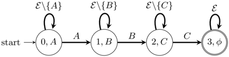
In this section, we present a generic algorithm for obtaining frequencies of episodes under the different frequency definitions listed in Sec. 2.1. The basic ingredient in all the algorithms is a simple Finite State Automaton (FSA) that is used to recognize (or track) an episode's occurrences in the event sequence.

The FSA for recognizing occurrences of ( A → B → C ) is illustrated in Fig. 1. In general, an FSA for an N -node serial episode α = α [1] → α [2] → . . . → α [ N ] has ( N +1) states. The first N states are represented by a pair ( i, α [ i + 1]), i = 0 , . . . N -1. The ( N +1) th state is ( N,φ ) where φ is a null symbol. Intuitively, if the FSA is in state ( j, α [ j +1]), it means that the FSA has already seen the first j event types of this episode and is now waiting for α [ j +1]; if we now encounter an event of type α [ j +1] in the data it can accept it (that is, it can transit to its next state). The start (first) state of the FSA is (0 , α [1]). The ( N +1) th state is the accepting state because when an automaton reaches this

state, a full occurrence of the episode is tracked.

We first explain how these FSA can be used for obtaining all the different types of frequencies of episodes before presenting the generic algorithm. While discussing various algorithms, we represent any occurrence h by [ t h ( v 1 ) , t h ( v 2 ) . . . t h ( v N ) ], which is the vector of times of the events that constitute the occurrence. For the discussion of all algorithms in this section, we consider the example of tracking occurrences of α = ( A → B → C → D ) in the data stream D 1 given by

There is a 'natural' lexicographic order on the set of all occurrences H , of any episode, α , defined below. This is a total order on H and it will be useful in our analysis.

/negationslash

Definition 8. The lexicographic ordering, < /star , on the set of all occurrences of α is defined as follows: h 1 < /star h 2 if the least i for which t h 1 ( v i ) = t h 2 ( v i ) is such that t h 1 ( v i ) < t h 2 ( v i ) .

The simplest of all automata-based frequency counting algorithms is the one for counting non-overlapped occurrences [10] which uses only 1-automata per episode. (We call it algorithm NO here). At the start, one automaton for each of the candidate episodes is initialized in its start state. Each of the automata make a state transition as soon as a relevant event-type appears in the data stream. Whenever an automaton reaches its final state, frequency of the corresponding episode is incremented, the automaton is removed from the system and a fresh automaton for the episode is initialized in the start state. As is easy to see, this method will count non-overlapped occurrences of episodes. Under the NO algorithm, we denote the occurrence tracked by the i th automaton initialized for α as h no i .

In our example, algorithm NO tracks the following two occurrences of the episode α : (i) h no 1 = [13715] and (ii) h no 2 = [19 21 25 29], and the corresponding non-overlapped frequency is 2.

In this paper we introduce the concept of earliest transiting occurrence of an episode which is useful for analyzing different frequency counting algorithms.

Definition 9. An occurrence h of α is called earliest transiting if E h ( v i ) is the first occurrence of α [ i ] after t h ( v i -1 ) ∀ i = 2 , 3 . . . N .

It is easy to see that all occurrences tracked by algorithm NO are earliest transiting. Let H e denote the set of all earliest transiting occurrences of a given episode. We denote the i th occurrence (as per the lexicographic ordering of occurrences)

in H e as h e i . There are 6 earliest transiting occurrences of α in D 1 . They are h e 1 = [1 3 7 15], h e 2 = [491115], h e 3 = [5 9 11 15], h e 4 = [14 17 20 23], h e 5 = [19 21 25 29] and h e 6 = [22 24 25 29]. The earliest transiting occurrences tracked by the NO algorithm are h no 1 = h e 1 and h no 2 = h e 5 .

While the algorithm NO is very simple and efficient, it can not handle any expiry-time constraint. Recall that the expirytime constraint specifies an upper-bound, T X , on the span of any occurrence that is counted. Suppose we want to count with T X = 9. Both the occurrences tracked by NO have spans greater than 9 and hence the resulting frequency count would be zero. However, h e 4 is an occurrence which satisfies the expiry time constraint. Algorithm NO can not track h e 4 because it uses only one automaton per episode and the automaton has to make a state transition as soon as the relevant event-type appears in the data. To overcome this limitation, the algorithm can be modified so that a new automaton is initialized in the start state, whenever an existing automaton moves out of its start state. All automata make state transitions as soon as they are possible. Each such automaton would track an earliest transiting occurrence. In this process, two automata may reach the same state. In our example, after seeing ( A, 5), the second and third automata to be initialized for α , would be waiting in the same state (ready to accept the next B in the data). Clearly, both automata will make state transitions on the same events from now on and so we need to keep only one of them. We retain the newer or most recently initialized automaton (in this case, the third automaton) since the span of the occurrence tracked by it would be smaller. When an automaton reaches its final state, if the span of the occurrence tracked by it is less than T X , then the corresponding frequency is incremented and all automata of the episode except the one waiting in the start state are retired. (This ensures we are tracking only non-overlapped occurrences). When the occurrence tracked by the automaton that reaches the final state fails the expiry constraint, we just retire the current automaton; any other automata for the episode will continue to accept events. Under this modified algorithm, in D 1 , the first automaton that reaches its final state tracks h e 3 which violates the expiry time constraint of T X = 9. So, we drop only this automaton. The next automaton that reaches its final state tracks h e 4 . This occurrence has span less than T X = 9. Hence we increment the corresponding frequency count and retire all current automata for this episode. Since there are no other occurrences non-overlapped with h e 4 , the final frequency would be 1. We denote this algorithm for counting the non-overlapped occurrences under an expirytime constraint as NO-X. The occurrences tracked by both NO and NO-X would be earliest transiting.

Note that several earliest transiting occurrences may end simultaneously. For example, in D 1 , h e 1 , h e 2 and h e 3 all end together at ( D, 15). Both { h e 2 , h e 5 } and { h e 3 , h e 6 } form maximal sets of non-overlapped occurrences. Sometimes (e.g. when determining the distribution of spans of occurrences for an episode) we would like to track the innermost one among the occurrences that are ending together. In this example, this means we want to track the set of occurrences { h e 3 , h e 6 } . This can be done by simply omitting the expirytime check in the NO-X algorithm. (That is, whenever an automaton reaches final state, irrespective of the span of the occurrence tracked by it, we increment frequency and retire all other automata except for the one in start state). We denote this as the NO-I algorithm and this is the algorithm proposed in [9].

In NO-I, if we only retire automata that reached their final states (rather than retire all automata except the one in the start state), we have an algorithm for counting minimal occurrences (denoted MO). In our example, the automata tracking h e 3 , h e 4 and h e 6 are the ones that reach their final states in this algorithm. The time-windows of these occurrences constitute the set of all minimal windows of α in D 1 . Expiry time constraints can be incorporated by incrementing frequency only when the occurrence tracked has span less than the expiry-time threshold. The corresponding expirytime algorithm is referred to as MO-X.

The windows-based counting algorithm (which we refer to as WB) is also based on tracking earliest transiting occurrences. WBalso uses multiple automata per episode to track minimal occurrences of episodes like in MO. The only difference lies in the way frequency is incremented. The algorithm essentially remembers, for each candidate episode, the last minimal window in which the candidate was observed. Then, at each time tick, effectively, if this last minimal window lies within the current sliding window of width T X , frequency is incremented by one. This is because, an occurrence of episode α exists in a given window w if and only w contains a minimal window of α .

It is easy to see that head frequency with a window-width of T X is simply the number of earliest transiting occurrences whose span is less than T X . Thus we can have a head frequency counting algorithm (referred to here as HD) that is similar to MO-X except that when two automata reach the same state simultaneously we do not remove the older automaton. This way, HD will track all earliest transiting occurrences which satisfy an expiry time-constraint of T X . For T X = 10 and for episode α , HD tracks h e 3 , h e 4 , h e 5 and h e 6 and returns a frequency count of 4. The total frequency count for an episode α is the minimum of the head frequencies of all its subepisodes (including itself). This can be computed as the minimum of the head frequency of α and the total frequency of its ( N -1)-suffix subepisodes which would have been computed in the previous pass over the data. (See [7] for details). The head frequency counting algorithm can have high space-complexity as all the time instants at which automata make their first state transition need to be remembered.

The non-interleaved frequency counting algorithm (which we refer to as NI) differs from the minimal occurrence algorithm in that, an automaton makes a state transition only if there is no other automaton of the same episode in the destination state. Unlike the other frequency counting algorithms discussed so far, such an FSA transition policy will track occurrences which are not necessarily earliest transiting. In our example, until the event ( A, 4) in the data sequence, both the minimal and non-interleaved algorithms make identical state transitions. However, on ( A, 5), NI will not allow the automaton in state (0 , A ) to make a state transition as there is already an active automaton for α in state (1 , B ) which had accepted ( A, 4) earlier. Eventually, NI tracks the occurrences h ni 1 = [1 3 7 15], h ni 2 = [4 9 16 18], h ni 3 = [14 17 20 23] and h ni 4 = [19 21 25 29].

While there are no algorithms reported for counting distinct occurrences, we can construct one using the same ideas. Such an algorithm (to be called as DO) differs from the one for counting minimal occurrences, in allowing multiple au- tomata for an episode to reach the same state. However, on seeing an event ( E i , t i ) which multiple automata can accept, only one of the automata (the oldest among those in the same state) is allowed to make a state transition; the others continue to wait for future events with the same event-type as E i to make their state transitions. The set of maximal distinct occurrences of α in D 1 are h d 1 = h e 1 , h d 2 = [4 9 11 18], h d 3 = [5 17 20 23], h d 4 = [14 21 25 29] and h d 5 = [19 24 30 31] which are the ones tracked by this algorithm.

We can also consider counting all occurrences of an episode even though it may be inefficient. The algorithm for counting all occurrences (referred to as the AO) allows all automata to make transitions whenever the appropriate events appear in the data sequence. However, at each state transition, a copy of the automaton in the earlier state is added to the set of active automata for the episode.

From the above discussion, it is clear that by manipulating the FSA (that recognize occurrences) in different ways we get counting schemes for different frequencies. The choices to be made in different algorithms essentially concern when to initiate a new automaton in the start state, when to retire an existing automaton, when to effect a possible state transition and when (and by how much) to increment the frequency. We now present a unified scheme incorporating all this in Algorithm 1 for obtaining frequencies of a set of serial episodes. This algorithm has five boolean variables, namely, TRANSIT, COPY-AUTOMATON, JOIN-AUTOMATON, INCREMENT-FREQ and RETIRE-AUTOMATON.The counting algorithms for all the different frequencies are obtained from this general algorithm by suitably setting the values of these boolean variables (either by some constants or by values calculated using the current context in the algorithm). Tables 2 - 6 specify the choices needed to obtain the algorithms for different frequencies. (A list of all algorithms is given in table 1).

As can be seen from our general algorithm, when an event type for which an automaton is waiting is encountered in the data, the the automaton can accept it only if the variable TRANSIT is true. Hence for all algorithms that track earliest transiting occurrences, TRANSIT will be set to true as can be seen from table 2. For algorithms NI and DO where we allow the state transition only if some condition is satisfied. The condition COPY-AUTOMATON (Table 3) is for deciding whether or not to leave another automaton in the current state when an automaton is transiting to the next state. Except for NO and AO, we create such a copy only when the currently transiting automaton is moving out of its start state. In NO we never make such a copy (because this algorithm uses only one automaton per episode) while in AO we need to do it for every state transition. As we have seen earlier, in some of the algorithms, when two automata for an episode reach the same state, the older automaton is removed. This is controlled by JOIN-AUTOMATON, as given by Table 4. INCREMENT-FREQUENCY (Table 5) is the condition under which the frequency of an episode is incremented when an automaton reaches its final state. This increment is always done for algorithms that have no expiry time constraint or window width. For the others we increment the frequency only if the occurrence tracked satisfies the constraint. RETIRE-AUTOMATA condition (Table 6) is concerned with removal of all automata of an episode when a complete occurrence has been tracked. This condition is true only for the non-overlapped occurrences-based counting algorithms.

Apart from the five boolean variables explained above, our general algorithm contains one more variable, namely, INC, which decides the amount by which frequency is incremented when an automaton reaches the final state. Its values for different frequency counts are listed in Table 7. For all algorithms except WB, we set INC = 1. We now explain how frequency is incremented in WB. To count the number of sliding windows that contain at least one occurrence of the episode, whenever a new minimal occurrence enters a sliding window, we can calculate the number of consecutive windows in which this new minimal occurrence will be found in. For example, in D 1 , with a windowwidth of T X = 16, consider the first minimal occurrence of ( A → B → C → D ), namely, the occurrence constituted by events ( A, 5), ( B, 9), ( C, 11) and ( D, 15). The first sliding window in which this occurrence can be found is [ -1 , 15]. The occurrence stays in consecutive sliding windows, until the sliding window [5 , 21]. When this first minimal occurrence enters the sliding window [ -1 , 15], we observe that there is no other 'older' minimal occurrence in [ -1 , 15], and hence, as per the else condition in Table 7 , the INC is incremented by (5 -( -1)+1) = 7. Similarly, when the second minimal occurrence enters the sliding window [7 , 23], we increment INC by (14 -7 + 1 = 8). The third minimal occurrence (constituted by the events ( A, 22), ( B, 24), ( C, 25) and ( D, 29)) first enters the sliding window [13 , 29], with the second minimal window still occurring within this window. This third minimal occurrence remains in consecutive sliding windows until [22 , 38]. As per the if condition of Table 7 , INC is incremented by 22 -14 = 8. We note that such an implementation of the windows-based algorithm removes the need for the beginsat ( t ) list of [14] which was used to store all automata whose first state transition occurred at time-tick t .

Remark 1. Even though we included AO (for counting all occurrences of an episode) for sake of completeness, this is not a good frequency measure. This is mainly because it does not seem to satisfy any anti-monotonicity condition. For example, consider the data sequence < AABBCC > . There are 8 occurrences of ( A → B → C ) but only 4 occurrences of each of its 2 -node subepisodes. Also, its space complexity can be high.

Remark 2. : The quantitative relationships between the different frequency counts for a given episode can be described as follows:

where f all denotes the frequency of an episode under AO, while f h and f tot denote the corresponding head and total frequencies defined with a window-width exceeding the total time-span of the event sequence. For a large sliding window width, the head frequency f h is same as the number of earliest transiting occurrences of an episode. In general, the inequality f d ≥ f ni holds only for injective episodes (An episode α is injective if it does not contain any repeated event-types). All other inequalities are true for any serial episode. The first inequality is obvious. The second inequality follows directly from equation 2 in definition 4 . Given a set of f maximal distinct occurrences of an episode α in a data stream D , one can extract that many earliest transiting

Table 1: Various frequency counts

WB	Windows based
MO	Minimal Occurrences based
MO-X	Minimal Occurrence with Expiry time constraints
NO	Non-overlapped
NO-I	Non-overlapped innermost
NO-X	Non-overlapped with Expiry time constraints
NI	Non-interleaved
DO	Distinct occurrences based
AO	All occurrences based
HD	Head frequency

Table 2: Conditions for TRANSIT=TRUE

WB, MO, MO-X, HD NO, NO-X, NO-I AO	Always
NI	If /notexistential earlier automaton for α in next state j
DO	No other earlier automaton for α waiting in same state can transit on event ( E i , t i ).

Table 3: Conditions for COPY-AUTOMATON=TRUE

WB, MO, MO-X, HD NI, NO-X, NO-I, DO	Only if A is in start state
NO	Never
AO	Always

Table 4: Conditions for JOIN-AUTOMATON=TRUE

WB, MO, MO-X, NO-X, NO-I	Always
DO, AO, HD, NO, NI	Never

Table 5: Conditions for INCREMENT-FREQ=TRUE

Table 6: Conditions for RETIRE-AUTOMATA=TRUE

MO, NO, NI, DO, AO, NO-I	Always
WB, NO-X MO-X, HD	If time difference between first and last state transitions is less than T X (window-width for WB, expiry time for others)

Table 7: Values taken by INC

NO, NO-X, NO-I	Always
WB, MO, MO-X HD, NI, DO, AO MO-X	Never

INC = 1 for all counts except WB.

For Windows Based count(WB),

If(first window which contains current minimal occurrence also contains the previous minimal occurrence), then

INC = Time diff. between start of last window containing the current minimal occurrence and the start of last window which contains previous minimal occurrence. else

INC=time difference between the first and last window containing the current occurrence +1.

Algorithm 1 Unified Algorithm for counting serial episodes

Input: Set C N of N -node serial episodes, event stream D = 〈 ( E 1 , t 1 ), . . . , ( E n , t n )) 〉 , Output: Frequencies of episodes in C N 1: for all α ∈ C N do 2: Add automaton of α waiting in the start state. 3: Initialize frequency of α to ZERO. 4: for l = 1 to n do 5: for each automaton, A , ready to accept event-type E i do 6: α =candidate associated with A ; 7: j = state which A is ready to transit into; 8: if TRANSIT then 9: if COPYAUTOMATON then 10: Add Copy of A to collection of automata. 11: Transit A to state j 12: if ∃ an earlier automaton of α already in state j but not waiting for E i then 13: if JOIN-AUTOMATON then 14: Retain A and retire earlier automaton 15: if A reached final state then 16: Retire A . 17: if INCREMENT-FREQ then 18: Increment frequency of α by INC. 19: if RETIRE-AUTOMATON then 20: Retire all automaton of α and create a state '0' automaton.

occurrences of not only α but also of all its subepisodes in D . Hence the third inequality is also true. Also, it is easy to verify that a set of non-interleaved occurrences of an injective episode are also distinct, which validates the fourth inequality. We will show the correctness of the remaining two inequalities in the next section.

4. PROOFS OF CORRECTNESS

In this section, we present proofs of correctness of the different frequency counting algorithms presented in Sec. 3 (all of which are specific instances of Algorithm 1 ).

In our proofs, we consider the case of event sequences with distinct occurrence-times for events. When we are not considering expiry-time constraints, the actual values of times of occurrences of different events are not really important; only the time ordering of the events is important in deciding on the occurrences of episodes. Hence, in this section we will use h ( v 1 ) interchangeably with t h ( v 1 ) , the time of the first event in the occurrence h and so on. Modifications needed in the case of data having multiple events with the same time of occurrence, are discussed at the end of the section.

4.1 Minimal Window Counting algorithm

First, we analyze the minimal occurrences counting algorithm (MO). Our proof methodology is different from the one presented in [4], where, the algorithm is viewed as computing a table S [0 . . . n, 0 . . . N ], where, S [ i, j ] is the largest value k ≤ i such that E k . . . E i contains an occurrence of α [1] → . . . α [ j ], using dynamic programming. The algorithm, after processing E i , stores the i th row of this matrix. The dynamic programming recursion helps compute the i th row of this matrix from its ( i -1) th row. Whenever S [ i, N ] > S [ i -1 , N ], the count is incremented since a new minimal occurrence is recognized. Viewed from an automata perspective, the i th row of the matrix essentially stores the first state transition times of the currently active automata. Our analysis of the minimal occurrence algorithm also leads to an analysis and proof for counting non-overlapped occurrences (NO and NO-X) as well. Another advantage of our proof strategy is that it may be generalized to the case of episodes with general partial orders. (We briefly discuss this in section 6).

Lemma 1. Suppose h is an earliest transiting occurrence of an N -node episode α . If h ′ is any general occurrence such that h < /star h ′ , then h ( v i ) ≤ h ′ ( v i ) ∀ i = 1 , 2 , . . . N .

This lemma follows easily from the definition of the lexicographic ordering, < /star , and the definition of earliest transiting occurrence.

Remark 3. Recall that h e i is the i th earliest transiting (ET) occurrence of an episode. Thus, by definition, h e i ( v 1 ) < h e j ( v 1 ) and h e i < /star h e j whenever i < j . Hence, from the above lemma, we have h e i ( v k ) ≤ h e j ( v k ) for all k and i < j . In particular, we have, h e i ( v 1 ) < h e i +1 ( v 1 ) and h e i ( v N ) ≤ h e i +1 ( v N ) , for an N -node episode.

The main idea of our proof is that to find all minimal windows of an episode, it is enough to capture a certain subset of earliest transiting occurrences.

Lemma 2. An earliest transiting (ET) occurrence h e i , of an N -node episode, is not a minimal occurrence if and only if h e i ( v N ) = h e i +1 ( v N ) .

Proof. The 'if' part follows easily from Remark 3. For the 'only if' part, let us denote by w = [ n s , n e ] = [ h e i ( v 1 ) , h e i ( v N )] the window of h e i . Given that w is not a minimal window, we need to show that h e i ( v N ) = h e i +1 ( v N ). Since w is not a minimal window, one of its proper sub-windows contains an occurrence, say, h , of this episode. That means if h starts at n s then it must end before n e . But, since h e i is earliest transiting, any occurrence starting at the same event as h e i can not end before h e i . Thus we must have h ( v 1 ) > h e i ( v 1 ). This means, by lemma 1, since h e i is earliest transiting, we can not have h e i ( v N ) > h ( v N ). Since the window of h has to be contained in the window of h e i , we thus have h e i ( v N ) = h ( v N ). By definition, h e i +1 will start at the earliest possible position after h e i . Since there is an occurrence starting with h ( v 1 ) we must have h e i +1 ( v 1 ) ≤ h ( v 1 ). Now, since h e i +1 is earliest transiting, it can not end after h . Thus we must have h e i +1 ( v N ) ≤ h ( v N ). Also, h e i +1 can not end earlier than h e i because both are earliest transiting. Thus, we must have h e i ( v N ) = h e i +1 ( v N ). This completes proof of lemma.

Remark 4. This lemma shows that any ET occurrence h e i such that h e i ( v N ) < h e i +1 ( v N ) is a minimal occurrence. The converse is also true. Consider a minimal window w = [ n s , n e ] . Since this is a minimal window, there is an occurrence (and hence an ET occurrence) starting at n s . Denote this ET occurrence by h e i . We know h e i ( v N ) = n e because w is a minimal window. Then the next ET occurrence h e i +1 has to start after n s and has to end beyond n e because w is minimal. Thus we have h e i ( v N ) < h e i +1 ( v N ) .

Now we are ready to prove correctness of the MO algorithm. Consider Algorithm 1 operating in the MO(minimal occurrence) mode for tracking occurrences of an N -node episode

α . Since TRANSIT is always true in the MO mode, all automata would be tracking ET occurrences. Since COPYAUTOMATON is true in MO mode whenever an automaton transits out of start state, we will always have an automaton in the start state. This, along with the fact that TRANSIT is always true, implies that the i th initialized automaton would be tracking h e i , the i th ET occurrence. Let us denote by A α i the i th initialized automaton. However, since JOIN-AUTOMATON is also always true, not all automata (initialized for this episode) would result in incrementing the frequency; some of them would be removed when one automaton transits into a state already occupied by some other automaton. In view of Lemma 2 and Remark 4, if we show that the automaton A α i results in increment of frequency if and only if h e i , the occurrence tracked by it, is such that h e i ( v N ) < h e i +1 ( v N ), then, the proof of correctness of MO algorithm is complete.

Lemma 3. In the MO algorithm the i th automaton that was initialized for α , referred to as A α i , contributes to the frequency count iff h e i ( v N ) < h e i +1 ( v N ) .

Proof.

A α i does not contribute to the frequency

• = ⇒ ∃ A α k , k > i, which transits into a state already occupied by A α i
• = ⇒ A α i is removed by a more recently initialized automaton
• = ⇒ ∃ k, j s.t. k > i, 1 < j ≤ N and h e i ( v j ) = h e k ( v j ) .

=

⇒ ∃

j

1

< j

≤

N s.t. h

e

i

(

v

j

) =

h

e

i

because, by Remark 3, for

e

e

e

i

h

=

⇒

h

+1

j

)

≤

h

(

v

j

)

≤

h

(

v

e

i

(

(

v

v

N

) =

i

h

e

i

+1

(

v

N

)

The last step follows because both h e i and h e i +1 are ET occurrences and hence h e i ( v j ) = h e i +1 ( v j ) implies h e i ( v j ′ ) = h e i +1 ( v j ′ ) , ∀ j ′ > j .

Conversely, we have

The first step follows because, if A α i contributes to the frequency then no automaton initialized after it would ever come to the same state occupied by it and since all occurrences tracked are earliest transiting, this must mean h e i ( v j ) < h e i +1 ( v j ), ∀ j . This completes proof of the lemma.

Another interesting observation is that if h e i is minimal, then it is non-interleaved with h e i +1 . Suppose h e i is minimal and h e i is not non-interleaved with h e i +1 . Since h e i is minimal, we have h e i ( v j ′ ) < h e i +1 ( v j ′ ) , ∀ j ′ . If h e i is not non-interleaved with h e i +1 , there exists a j < N such that h e i +1 ( v j ) < h e i ( v j +1 ). Thus we must have h e i ( v j ) < h e i +1 ( v j ) < h e i ( v j +1 ) < h e i +1 ( v j +1 ). But this can not be because E h e i ( v j +1 ) is the earliest α [ j + 1] after h e i ( v j ) and if it is also after h e i +1 ( v j ) then the fact that both h e i and h e i +1 are ET occurrences should mean h e i ( v j +1 ) = h e i +1 ( v j +1 ) which contradicts that h e i is minimal. Hence h e i and h e i +1 are noninterleaved.

Thus, given the sequence of minimal windows, the earliest transiting occurrences from each of these minimal windows gives a sequence of (same number of) non-interleaved occurrences. This leads to f mi ≤ f ni as stated earlier in (3).

k

j

)

,

+1

(

v

j

)

.

k > i,

∀

j

4.2 Other ET occurrences-based algorithms

4.2.1 Proofs of correctness for NO-X and NO-I

The NO-X algorithm can be viewed as a slight modification to the MO algorithm. As in the MO algorithm, we always have an automaton in the start state and all automata make transitions as soon as possible and when an automaton transits into a state occupied by another, the older one is removed. However, in the NO-X algorithm, the INCREMENT-FREQ variable is true only when we have an occurrence satisfying T X constraint. Hence, to start with, we look for the first minimal occurrence which satisfies the expiry time constraint and increment frequency. At this point, (unlike in the MO algorithm) we terminate all automata except the one in the start state since we are trying to construct a non-overlapped set of occurrences. Then we look for the next earliest minimal occurrence (which will be non-overlapped with the first one) satisfying expiry time constraint and so on. Since minimal occurrences locally have the least time span, this strategy of searching for minimal occurrences satisfying expiry time constraint in a non-overlapped fashion is quite intuitive. Let H nX = { h nX 1 , h nX 2 . . . h nX f ′ } denote the sequence of occurrences tracked by the NO-X algorithm (for an N -node episode). Then the following property of H nX is obvious.

Property 1. h nX 1 is the earliest minimal occurrence satisfying expiry time constraints. h nX i is the first minimal occurrence (satisfying expiry time constraint) that starts after h nX i -1 ( v N ) . There is no minimal occurrence satisfying expiry time constraint which starts after h nX f ′ ( v N ) .

Theorem 1. H nX is a maximal non-overlapped sequence satisfying expiry time constraint T X .

Proof. Consider any other set of non-overlapped occurrences satisfying expiry constraints, H ′ = { h ′ 1 , h ′ 2 . . . h ′ l } such that h ′ i < /star h ′ i +1 . Let m = min { f ′ , l } . Then we first show

Suppose h ′ 1 ( v N ) < h nX 1 ( v N ). Consider the earliest transiting occurrence h ′′ starting from h ′ 1 ( v 1 ). This ends at or before h ′ 1 ( v N ) by lemma 1. Among all ET occurrences that end at the same event as h ′′ , the last one (under the lexicographic ordering) is a minimal occurrence by lemma 2. Its window is contained in that of h ′ 1 which satisfies the expiry time constraint. Hence we have found a minimal occurrence satisfying expiry constraint ending before h nX 1 which contradicts the first statement of property 1. Hence h nX 1 ( v N ) ≤ h ′ 1 ( v N ). Now applying the same argument to the data stream starting with the first event after h nX 1 ( v N ), we get h nX 2 ( v N ) ≤ h ′ 2 ( v N ) and so on and thus can conclude h nX i ( v N ) ≤ h ′ i ( v N ) ∀ i . This shows that no other set of non-overlapped occurrences can have more number of occurrences than those in H nX . Hence, H nX is maximal.

If we choose T X equal to the time span of the data stream, the NO-X algorithm reduces to the NO-I algorithm because every occurrence satisfies expiry constraint. Hence proof of correctness of NO-I algorithm is immediate.

4.2.2 Relation between NO-I and NO algorithms

We now explain the relation between the sets of occurrences tracked by the NO and NO-I algorithms. As proved in [10]

the NO algorithm (which uses one automaton per episode), tracks a maximal non-overlapped sequence of occurrences, say, H no = { h no 1 , h no 2 . . . h no f no } . Since the NO-I algorithm has no expiry time constraint, it also tracks a maximal set of non-overlapped occurrences. Among all the ET occurrences that end at h no i ( v N ), let h in i be the last one (as per the lexicographic ordering). Then the i th occurrence tracked by the NO-I algorithm would be h in i as we show now. Since h no 1 would be the first ET occurrence, it is clear from our discussion in the previous subsection that the first occurrence tracked by the MO algorithm would be h in 1 . As is easy to see, the MO and NO-I algorithms would be identical till the first time an automaton reaches the accepting state. Hence h in 1 would be the first occurrence tracked by the NO-I algorithm. Now the NO-I algorithm would remove all automata except for the one in the start state. Hence, it is as if we start the algorithm with data starting with the first event after h no 1 ( v N ) = h in 1 ( v N ). Now, by the property of NO algorithm, h no 2 would be the first ET occurrence in this data stream and hence h in 2 would be the first minimal window here. Hence it is the second occurrence tracked by NO-I and so on.

The above also shows that each occurrence tracked by the NO-I algorithm is also tracked by the MO algorithm and hence we have f no ≤ f mi as stated in (3). H in is also a maximal set of non-overlapping minimal windows as discussed in [21].

4.3 Non-interleaved and Distinct Occurrences based Algorithms

The algorithm NI which counts non-interleaved occurrences is different from all the ones discussed so far because it does not track ET occurrences. Here also we always have an automaton waiting in the start state. However, the transitions are conditional in the sense that the i th created automaton makes a transition from state ( j -1) to j provided the ( i -1) th created automaton is past state j after processing the current event. This is because we want the i th automata to track an occurrence non-interleaved with the occurrence tracked by ( i -1) th automaton. Let H ni = { h ni 1 , h ni 2 , . . . h ni f ′ } be the sequence of occurrences tracked by NI. From the above discussion it is clear that it has the following property (while counting occurrences of α ).

Property 2. h ni 1 is the first or earliest occurrence (of α ). For all i > 1 and ∀ j = 1 , . . . , N -1, h ni i ( v j ) is the first occurrence of α [ j ] at or after h ni i -1 ( v j +1 ); and h ni i ( v N ) is the earliest occurrence of α [ N ] after h ni i ( v N -1 ). There is no occurrence of α beyond h ni f ′ which is non-interleaved with it.

The proof that H ni is a maximal non-interleaved sequence is very similar in spirit to that of the NO-X algorithm. As earlier, we can show that given an arbitrary sequence of non-interleaved occurrences H ′ = { h ′ 1 , h ′ 2 . . . h ′ l } , we have h ni i ( v k ) ≤ h ′ i ( v k ) , ∀ i, k and hence get the correctness proof of NI algorithm. It is easy to verify the correctness of the DO algorithm also along similar lines.

It appears difficult to extend both the NI and DO algorithms to incorporate expiry time constraints. For this we should track a set of occurrences h 1 , h 2 . . . of α , where h 1 is the first occurrence satisfying T X and h 2 is the next earliest occurrence satisfying T X that is non-interleaved with (or distinct from, in case of DO) h 1 and so on. Note that this h 2 need not have to be the earliest occurrence non-overlapped with h 1 . At present, there are no algorithms for counting non-interleaved or distinct occurrences satisfying an expiry time constraint.

Before ending this section, we briefly outline what needs to be done when the data stream contains multiple events having the same time of occurrence. An important thing to note is that two events having the same time of occurrence cannot be a part of a serial episode occurrence. Hence, each automata can at most accept one event from a set of events having the same occurrence time. With this condition, the DO, AO and HD algorithms go through as before. One would need to process the set of events having the same occurrence time together and allow all the permissible automata to make a one step transition first as done using transitions () list in [14]. After this, before processing the set of events with the next occurrence time, we would need to do the multiple automata check for the various candidate episodes and delete the appropriate older automata for algorithms MO, MO-X, NO-I and NO-X. For the non-interleaved algorithm, one needs to actually back track the transitions which resulted in two automata to coalesce.

5. CANDIDATE GENERATION

In this section, we discuss the anti-monotonicity properties of the various frequency counts, which in-turn are exploited by their respective candidate generation steps in the Apriori- style level-wise procedure for frequent episode discovery. It is well known that the windows-based [14], non-overlapped [9] and total [7] frequency measures satisfy the anti-monotonicity property that all subepisodes of a frequent episode are frequent . One can verify that the same holds for the distinct occurrences based frequency too. It has been pointed out in [7] that the head frequency does not satisfy this antimonotonicity property. For an episode α , in general, only the subepisodes involving α [1] are as frequent as α under the head count. In a level-wise apriori-based episode discovery, the candidate generation for the head frequency count would exploit the condition that if an N -node episode is frequent, then all ( N -1)-node subepisodes that include α [1] have to be frequent. The head frequency definition has some limitations in the sense that the frequency of the ( N -1)node suffix subepisode 2 can be arbitrarily low. Consider the event stream with 100 A s followed by a B and C . Suppose all occurrences of A → B → C satisfy the expiry constraint T X . Even though there are 100 occurrences of A → B → C , there is only one occurrence of B → C . This can be a problem when one desires that the frequent episodes capture repetitive causative influences.

Like the head frequency, the minimal occurrences (windows) and the non-interleaved occurrences also do not satisfy the anti-monotonicity property that all subepisodes are at least as frequent as the corresponding episode. However, the ( N -1)-node prefix and suffix subepisodes are at least as frequent as the episode as we show below. For an example, consider a data stream where successive events are given by ABACBDCD . Even though there are two minimal win-

2 Given an N -node episode α [1] → α [2] → ·· · → α [ N ], its K -node prefix subepisode is α [1] → α [2] → ··· → α [ k ] and its ( N -K )-node suffix subepisode is α [ K +1] → α [ K +2] → · · ·→ α [ N ] for K = 1 , 2 , · · · , ( N -1).

dows (and two non-interleaved occurrences) of A → B → C → D , there is only one minimal window (and one noninterleaved occurrence) of each of the non-prefix and nonsuffix subepisodes A → B → D and A → C → D . However, the situation here is not as bad as that for head frequency because all such subepisodes will have at least as many distinct occurrences as the number of minimal or noninterleaved occurrences of the episode, at least in case of injective episodes. (Note that this example is that of an injective episode). This is because, in case of injective episodes, the number of distinct occurrence is always greater than the non-interleaved count, which in-turn is greater than the minimal windows count. Hence, given that there are f noninterleaved or minimal occurrences of an injective episode α , there are at least f distinct occurrences of α too. Since the distinct occurrences based frequency satisfies the original anti-monotonicity property, all subepisodes of α too will have at least f distinct occurrences.

We now formally prove the anti-monotonicity property for minimal and non-interleaved occurrences based frequencies.

Theorem 2. If a N-node serial episode α has a frequency f in the minimal or the non-interleaved sense, then its ( N -1) -prefix subepisode ( α p ) and suffix subepisode ( α s ) have a frequency of at least f .

Proof. Consider a minimal window of the episode α , w = [ n s , n e ]. Consider the earliest occurrence h p of the prefix subepisode starting from n s and let w ′ be its window. Any proper sub-window of w ′ starting at n s and containing an occurrence of α p contradicts lemma 1. A proper subwindow of w ′ containing an occurrence of α p starting after n s would contradict the minimality of w itself. Hence w ′ is a minimal window of α p starting at n s . We hence conclude that α p has a frequency of at least f . A similar proof works for the suffix subepisode by considering the window of the last occurrence h s of the suffix subepisode ending at n e .

Let H ni = { h 1 , h 2 , . . . h f } be a maximal non-interleaved sequence. From each occurrence h k , we choose the suboccurrence h ′ k = [ h k ( v 1 ) , h k ( v 2 ) , . . . h k ( v N -1 ], of α p . It is easy to see that this new sequence of occurrences h ′ 1 , h ′ 2 , . . . h ′ f forms a non-interleaved sequence. Hence the frequency of α p is at least f . A similar argument works for the suffix episode.

Hence, for every episode α , we extract its ( N -1) suffix, go down the candidate list and search for a block of episodes whose N -1 prefix matches this suffix. We form candidates as many as the number of episodes in this matching block. This kind of candidate generation has already been reported in the literature in [20], [18] and [19] in the context of sequences under inter-event time constraints.

6. DISCUSSION AND CONCLUSIONS

The framework of frequent episodes in event streams is a very useful data mining technique for unearthing temporal dependencies from data streams in many applications. The framework is about a decade old and many different frequency measures and associated algorithms have been proposed over the last ten years. In this paper we have presented a generic automata-based algorithm for obtaining frequencies of a set of candidate episodes. This method unifies all the known algorithms in the sense that we can particularize our algorithm (by setting values for a set of variables) for counting frequent episodes under any of the frequency measures proposed in literature.

As we showed here, this unified view gives useful insights into the kind of occurrences counted under different frequency definitions and thus also allows us to prove relations between frequencies of an episode under different frequency definitions. Our view also allows us to get correctness proofs for all algorithms. We introduced the notion of earliest transiting occurrences and, using this concept, are able to get simple proofs of correctness for most algorithms. This has also allowed us to understand the kind of anti-monotonicity properties satisfied by different frequency measures.

While the main contribution of this paper is this unified view of all frequency counting algorithms, some of the specific results presented here are also new. The relationships between different frequencies of an episode (cf. eqn 3), is proved here for the first time. The distinct-occurrences based frequency and an automata-based algorithm for it are novel. The specific proof of correctness presented here for minimal occurrences is also novel. Also, the correctness proofs for non-overlapped occurrences based frequency counting under expiry time constraint has been provided here for the first time.

In this paper we have considered only the case of serial episodes. This is because, at present, there are no algorithms for discovering general partial orders under the various frequency definitions. However, all counting algorithms explained here for serial episodes can be extended to episodes with a general partial order structure. We can come up with a similar finite state automata(FSA) which track the earliest transiting occurrences of an episode with a general partial order structure [1]. For example, consider a partial order episode ( AB ) → C which represents A and B occurring in any order followed by a C . In order to track an occurrence of such a pattern, the initial state has to wait for either of A and B . On seeing an A it goes to state-1 where it waits only for a B ; on the other hand, on seeing a B first it moves to state-2 where it waits only for an A . Then on seeing a B in state-1 or seeing a A in state-2 it moves into state-3 where it waits for a C and so on. Thus, in each state in such a FSA, in general, we wait for any of a set of event types (instead of a single event for serial episodes) and a given state will now branch out into different states on different event types. With such a FSA technique it is possible to generalize the method presented here so that we have algorithms for counting frequencies of general partial order episodes under different frequencies. The proofs presented here for serial episodes can also be extended for general partial order episodes. While it seems possible, as explained above, to generalize the counting schemes to handle general partial order episodes, it is not obvious what would be an appropriate candidate generation scheme for general partial order episodes under different frequency definitions. This is an important direction for future work.

In this paper, we have considered only expiry time constraint which prescribes an upper bound on the span of the occurrence. It would be interesting to see under what other time constraints (e.g., gap constraints), design of counting algorithms under this generic framework is possible. Also, some unexplored choice of the boolean conditions in the proposed generic algorithm may give rise to algorithms for new use- ful frequency measures. This is also a useful direction of research to explore.

7. REFERENCES

1. Avinash Achar, Srivatsan Laxman, V. Raajay, and P. S. Sastry. Discovering general partial orders from event streams. Technical Report arXiv: 0902.1227v2 [cs.AI] http://arxiv.org, Dec 2009.
2. Bouchra Bouqata, Christopher D. Caraothers, Boleslaw K. Szymanski, and Mohammed J. Zaki. Vogue: A novel variable order-gap state machine for modeling sequences. In Proc. European Conf. Principles and Practice of Knowledge Discovery in Databases (PKDD'06) , pages 42-54, Sep 2006.
3. G. Casas-Garriga. Discovering unbounded episodes in sequential data. In Proc. European Conf. Principles and Practice of Knowledge Discovery in Databases (PKDD'03) , pages 83-94, Sep 2003.
4. G. Das, R. Fleischer, L. G¸ asieniec, D. Gunopulos, and J. K¨ arkk¨ ainen. Episode matching. In Proc. Annual Symp. Combinatorial Pattern Matching(CPM'97) , pages 12-27, Jun-July 1997.
5. R. Gwadera, M. J. Atallah, and W. Szpankowski. Reliable detection of episodes in event sequences. In Proc. IEEE Int'l Conf. Data Mining (ICDM'03) , pages 6774, Nov 2003.
6. Kuo-Yu Huang and Chia-Hui Chang. Efficient mining of frequent episodes from complex sequences. Information Systems , 33(1):96-114, Mar 2008.
7. Iwanuma K., Takano Y., and Nabeshima H. On antimonotone frequency measures for extracting sequential patterns from a single very-long sequence. In Proc. IEEE Conf. Cybernetics and Intelligent Systems , pages 213-217, Dec 2004.
8. Srivatsan Laxman. Discovering frequent episodes: Fast algorithms, Connections with HMMs and generalizations . PhD thesis, Bangalore, India, Sep 2006.
9. Srivatsan Laxman, P. S. Sastry, and K. P. Unnikrishnan. Discovering frequent episodes and learning Hidden Markov Models: A formal connection. IEEE Transactions on Knowledge and Data Engineering , 17(11):1505-1517, November 2005.
10. Srivatsan Laxman, P. S. Sastry, and K. P. Unnikrishnan. A fast algorithm for finding frequent episodes in event streams. In Proc. ACM SIGKDD Int'l Conf. Knowledge Discovery and Data Mining (KDD'07) , pages 410-419, Aug 2007.
11. Srivatsan Laxman, Vikram Tankasali, and Ryen W. White. Stream prediction using a generative model based on frequent episodes in event sequences. In Proc. ACM SIGKDD Int'l Conf. Knowledge Discovery and Data Mining (KDD'09) , pages 453-461, Jul 2008.
12. Jianxiong Luo and Susan Bridges, M. Mining fuzzy association rules and fuzzy frequent episodes for intrusion detection. International Journal of Intelligent Systems , 15(8):687-703, Jun 2000.
13. H. Mannila and H. Toivonen. Discovering generalized episodes using minimal occurrences. In Proc. Int'l Conf. Knowledge Discovery and Data Mining (KDD'96) , pages 146-151, August 1996.
14. Heikki Mannila, Hannu Toivonen, and A. Inkeri Verkamo. Discovery of frequent episodes in event sequences. Data Mining and Knowledge Discovery , 1(3):259-289, 1997.
15. Nicolas Meger and Christophe Rigotti. Constraintbased mining of episode rules and optimal window sizes. In Proc. European Conf. Principles and Practice of Knowledge Discovery in Databases (PKDD'04) , September 2004.
16. Fabian Morchen. Unsupervised pattern mining from symbolic temporal data. In SIGKDD Explorations , volume 9, pages 41-55, jun 2007.
17. Anny Nag and Ada Fu, Wai-chee. Mining freqeunt episodes for relating financial events and stock trends. In Proc. Pacific-Asia Conf. Knowledge Discovery and Data Mining, (PAKDD 2003) , pages 27-39, 2003.
18. Salvatore Orlando, Raffaele Perego, and Claudio Silvestri. A new algorithm for gap constrained sequence mining. In Proc. ACM symp. Applied computing , pages 540-547, mar 2004.
19. Debprakash Patnaik, P. S. Sastry, and K. P. Unnikrishnan. Inferring neuronal network connectivity from spike data: A temporal data mining approach. Scientific Programming , 16(1):49-77, Jan 2007.
20. R. Srikanth and R. Agrawal. Mining sequential patterns: Generalizations and performance improvements. In Proc. Int'l Conf. Extending Database Technology (EDBT) , March 1996.
21. Nikolaj Tatti. Significance of episodes based on minimal windows. In Proc. IEEE Int'l Conf. Data Mining(ICDM'09) , Dec 2009.
22. K. P. Unnikrishnan, Basel Q. Shadid, P. S. Sastry, and Srivatsan Laxman. Root cause diagnostics using temporal datamining. U.S.Patent no. 7509234, 24 Mar 2009.
23. Min-Feng Wang, Yen-Ching Wu, and Meng-Feng Tsai. Exploiting frequent episodes in weighted suffix tree to improve intrusion detection system. In Proc. Int'l Conf. Advanced Information Networking and Applications(AINA'08) , pages 1246-1252, Mar 2008.