A Unifying Probabilistic Perspective for Spectral Dimensionality Reduction: Insights and New Models

Neil D. Lawrence ∗ Sheffield Institute for Translational Neuroscience and Department of Computer Science University of Sheffield

[email protected]

October 26, 2018

Abstract

We introduce a new perspective on spectral dimensionality reduction which views these methods as Gaussian Markov random fields (GRFs). Our unifying perspective is based on the maximum entropy principle which is in turn inspired by maximum variance unfolding. The resulting model, which we call maximum entropy unfolding (MEU) is a nonlinear generalization of principal component analysis. We relate the model to Laplacian eigenmaps and isomap. We show that parameter fitting in the locally linear embedding (LLE) is approximate maximum likelihood MEU. We introduce a variant of LLE that performs maximum likelihood exactly: Acyclic LLE (ALLE). We show that MEU and ALLE are competitive with the leading spectral approaches on a robot navigation visualization and a human motion capture data set. Finally the maximum likelihood perspective allows us to introduce a new approach to dimensionality reduction based on L1 regularization of the Gaussian random field via the graphical lasso.

1 Introduction

A representation of an object for processing by computer typically requires that object to be summarized by a series of features, represented by numbers. As the representation becomes more complex, the number of features required typically increases. Examples include: the characteristics of a customer in a database; the pixel intensities in an image; a time series of angles associated with data captured from human motion for animation; the energy at different frequencies (or across the cepstrum) as a time series for interpreting speech; the frequencies of given words as they appear in a set of documents; the level of expression of thousands of genes, across a time series, or for different diseases.

With the increasing complexity of the representation, the number of features that are stored also increases. Data of this type is known as high dimensional data.

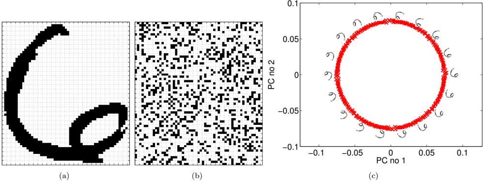
Consider the simple example of a handwritten six. The six in figure 1 is represented on a grid of pixels which is 64 rows by 57 columns, giving a datum with 3,648 dimensions. The space in which this digit sits contains far more than the digit. Imagine a simple probabilistic model of the digit which assumes that each pixel in the image is independent and is on with a given probability. We can sample from such a model (figure 1(b)).

Even if we were to sample every nanosecond from now until the end of the universe we would be highly unlikely to see the original six. The space covered by this model is very large but fundamentally the data lies on low dimensional embedded space. This is illustrated in figure 1(c). Here a data set has been constructed by rotating the digit 360 times in one degree intervals. The data is then projected onto its first two principal components. The spherical structure of the rotation is clearly visible in the projected data. Despite the data being high dimensional, the underlying structure is low dimensional. The objective of dimensionality reduction is to recover this underlying structure.

∗ Work also carried out at the School of Computer Science, University of Manchester.

Given a data set with n data points and p features associated with each data point, dimensionality reduction involves representing the data set using n points each with a reduced number, q , of features, with q < p . Dimensionality reduction is a popular approach to dealing with high dimensional data: the hope is that while many data sets seem high dimensional, it may be that their intrinsic dimensionality is low like the rotated six above.

1.1 Spectral Dimensionality Reduction

Spectral approaches to dimensionality reduction involve taking a data set containing n points and forming a matrix of size n × n from which eigenvectors are extracted to give a representation of the data in a low dimensional space. Several spectral methods have become popular in the machine learning community including isomap [Tenenbaum et al., 2000], locally linear embeddings [LLE, Roweis and Saul, 2000], Laplacian eigenmaps [Belkin and Niyogi, 2003] and maximum variance unfolding [MVU, Weinberger et al., 2004]. These approaches (and kernel principal component analysis [kernel PCA, Sch¨ olkopf et al., 1998]) are closely related to classical multidimensional scaling [CMDS, Mardia et al., 1979]. For a kernel perspective on the relationships see Ham et al. [2004], Bengio et al. [2004b,a].

In classical multidimensional scaling an n × n symmetric distance matrix, whose elements contain the distance between two data points, is converted to a similarity matrix and visualized through its principal eigenvectors. Viewed from the perspective of CMDS the main difference between the spectral approaches developed in the machine learning community is in the distance matrices they (perhaps implicitly) proscribe.

In this paper we introduce a probabilistic approach to constructing the distance matrix: maximum entropy unfolding (MEU). We describe how isomap, LLE, Laplacian eigenmaps and MVU are related to MEU using the unifying perspective of Gaussian random fields and CMDS.

The parameters of the model are fitted through maximum likelihood in a Gaussian Markov random field (GRF). The random field specifies dependencies between data points rather than the more typical approach which specifies dependencies between data features . We show that the locally linear embedding algorithm is an approximation to maximum entropy unfolding where pseudolikelihood is maximized as an approximation to the model likelihood. Our probabilistic perspective inspires new dimensionality reduction algorithms. We introduce an exact version of locally linear embedding based on an acyclic graph structure that maximizes the true model likelihood (acyclic locally linear embedding, ALLE). We also consider approaches to learning the structure of the GRF through graphical regression, [Friedman et al., 2008]. By L1 regularization of the dependencies we explore whether learning the graph structure (rather than prespecifying by nearest neighbour) improves performance. We call the algorithm Dimensionality reduction through Regularization of the Inverse covariance in the Log Likelihood (DRILL).

Our methods are based on maximum likelihood. Normally maximum likelihood algorithms specify a distribution which factorizes over the data points (each data point is independent given the model parameters). In our models the likelihood factorizes over the features (each feature from the data set is independent given the model parameters). This means that maximum likelihood in our model is consistent as the number of features increases, p →∞ rather than the number of data points. Alternatively, the parameters of our models become better determined as the number of features increase, rather than the number of data. This leads to a blessing of dimensionality where the parameters are better determined as the number of features increases. This has significant implications for learning in high dimensional data (known as the large p small n regime) which run counter to received wisdom.

In Section 2 we derive our model through using standard assumptions from the field of dimensionality reduction and the maximum entropy principle [Jaynes, 1986]. We then relate the model to other popular spectral approaches for dimensionality reduction and show how the parameters of the model can be fitted through maximum likelihood. This allows us to regularize the system with sparse priors and seek MAP solutions that restrict the inter point dependencies. Finally, we demonstrate the model (with comparisons) on two real world data sets. First though, we will review classical multidimensional scaling which provides the general framework through which these approaches can be related [see also Ham et al., 2004, Bengio et al., 2004b,a].

1.2 Classical Multidimensional Scaling

Given an n × n matrix of similarities, K , or dissimilarities, D , between a set of data points, multidimensional scaling considers the problem of how to represent these data in a low dimensional space. One way of doing this is to associate a q dimensional latent vector with each data point, y i, : , and define a set of dissimilarities between each latent point, δ i,j = ‖ x i, : -x j, : ‖ 2 2 (where ‖·‖ 2 represents the L2-norm) to give a matrix ∆ . Here we have specified the squared distance between each point as the dissimilarity. 1

If the error for the latent representation is then taken to be the sum of absolute values between the dissimilarity matrix entries,

and we assume that the data dissimilarities also represent a squared Euclidean distance matrix (perhaps computed in some high, maybe infinite, dimensional space) then the optimal linear dimensionality reduction is given by the following procedure [Mardia et al., 1979, pg 400],

1. Convert the matrix of dissimilarities to a matrix of similarities by taking B = -1 2 HDH where H = I -n -1 11 glyph[latticetop] is a centering matrix.
2. Extract the first q principal eigenvectors of B .
3. Setting X to these principal eigenvectors (appropriately scaled) gives a global minimum for the error function (1).

The centering matrix H is so called because when applied to data in the form of a design matrix, Y , i.e. one where each row is a data point and each column is a data set feature, the centred data matrix is recovered,

where µ = n -1 Y1 is the empirical mean of the data set.

2 Maximum Entropy Unfolding

Classical multidimensional scaling provides the optimal linear transformation of the space in which the squared distances are expressed. The key contribution of recently developed spectral approaches in machine learning is to compute these distances in a space which is nonlinearly related to the data thereby ensuring a nonlinear dimensionality reduction algorithm. From a machine learning perspective this is perhaps clearest for kernel PCA [Sch¨ olkopf

1 It is more usual to specify the distance directly as the dissimilarity, however, for our purposes it will be more convenient to work with squared distances

et al., 1998]. In kernel PCA the squared distances are computed between points in a Hilbert space and related to the original data through a kernel function,

For the linear kernel function, k ( y i, : , y j, : ) = y glyph[latticetop] i, : y j, : this reduces to the squared Euclidean distance, but for nonlinear kernel functions such as k ( y i, : , y j, : ) = exp( -γ ‖ y i, : -y j, : ‖ 2 2 ) the distances are nonlinearly related to the data space. They are recognized as squared distances which are computed in a 'feature space' [see e.g. Ham et al., 2004, Bengio et al., 2004b,a]. If we equate the kernel matrix, K , to the similarity matrix in CMDS then this equation is also known as the standard transformation between a similarity and distance [Mardia et al., 1979].

Kernel PCA (KPCA) recovers an x i, : for each data point and a mapping from the data space to the X space. Under the CMDS procedure we outlined above the eigenvalue problem is performed on the centered kernel matrix,

B = HKH ,

where K = [ k ( y i, : , y j, : )] i,j . This matches the procedure for the KPCA algorithm [Sch¨ olkopf et al., 1998] 2 . However, for the commonly used exponentiated quadratic kernel,

KPCA actually expands the feature space rather than reducing the dimension [see Weinberger et al., 2004, for some examples of this]. Unless data points are repeated the exponentiated quadratic kernel always leads to a full rank matrix, K , and correspondingly a rank n -1 centred kernel matrix, B . To exactly reconstruct the squared distances computed in feature space all but one of the eigenvectors of B need to be retained for our latent representation, X . If the dimensionality of the data, p , is smaller than the number of data points, n , then we have a latent representation for our data which has higher dimensionality than the original data.

The observation that KPCA doesn't reduce the data dimensionality motivated the maximum variance unfolding algorithm [MVU, Weinberger et al., 2004]. The idea in MVU is to learn a kernel matrix that will allow for dimensionality reduction. This is achieved by only considering local relationships in the data. A set of neighbors is defined (e.g. by k -nearest neighbors) and only distances between neighboring data points are respected. These distances are specified as constraints, and the other elements of the kernel matrix are filled in by maximizing its trace, tr ( K ), i.e. the total variance of the data in feature space, while respecting the distance constraints and keeping the resulting matrix centered. Maximizing tr ( K ) maximizes the interpoint squared distances for all points that are unconnected in the neighborhood graph, thereby unravelling the manifold.

In this paper we consider an alternative maximum entropy formalism of this problem. Since entropy is related to variance, we might expect a similar result in the quality of the resulting algorithm, but since maximum entropy also provides a probability distribution we should also obtain a probabilistic model with all the associated advantages (dealing with missing data, extensions to mixture models, fitting parameters by Bayesian methods, combining with other probabilistic models). Importantly, our interpretation will also enable us to relate our algorithm to other well known spectral techniques as they each turn out to approximate maximum entropy unfolding in some way.

2.1 Constraints from D Lead to a Density on Y

The maximum entropy formalism [see e.g. Jaynes, 1986] allows us to derive a probability density given only a set of constraints on expectations under that density. These constraints may be derived from observation. In our case the observations will be squared distances between data points, but we will derive a density over Y directly (not over the squared distances). We will do this by looking to constrain the expected squared inter-point distances, d i,j , of any two samples, y i, : and y j, : , from the density. This means that while our observations may be only of the squared distances, d i,j , the corresponding density will be over the data space that gives rise to those distances, p ( Y ). Of course, once we have found the form of probability density we are free to directly model in the space Y or make use only of the squared distance constraints. Direct modeling in Y turns out to be equivalent to maximum likelihood. However, since we do not construct a density over the squared distance matrix, modeling based on that information alone should be thought of as maximum entropy under distance constraints rather than maximum likelihood.

Maximum entropy is a free form optimization over all possible forms for the density given the moment constraints we impose. In the maximum entropy formalism, we specify the density by a free form maximization of the entropy subject to the imposed expectation constraints. The constraints we use will correspond to the constraints applied to maximum variance unfolding: the expectations of the squared distances between two neighboring data points sampled from the model.

2 For stationary kernels, kernel PCA also has an interpretation as a particular form of metric multidimensional scaling, see Williams [2001] for details.

2.2 Maximum Entropy in Continuous Systems

The entropy of a continuous density is normally defined as the limit of a discrete system. The continuous distribution is discretized and we consider the limit as the discrete bin widths approach zero. However, as that limit is taken the a term dependent on the bin width approaches ∞ . Normally this is dealt with by ignoring that term and referring to the remaining term as differential entropy. However, the maximum entropy solution for this differential entropy turns out to be undefined. Jaynes proposes an alternative invariant measure to the entropy. For maximum entropy in continuous systems we maximize the negative Kullback Leibler divergence [KL divergence, Kullback and Leibler, 1951] between a base density, m ( Y ), and the density of interest, p ( Y ),

Maximizing this measure is equivalent to minimizing the KL divergence between p ( Y ) and the base density, m ( Y ). Any choice of base density can be made, but the solution will be pulled towards the base density (through the minimization of the KL divergence). We choose a base density to be a very broad, spherical, Gaussian density with covariance γ -1 I . This adds a new parameter, γ , to the system, but it will turn out that this parameter has little affect on our analysis. Typically it can be taken to zero or assumed small. The density that minimizes the KL divergence under the constraints on the expectations is then

where N ( i ) represents the set of neighbors of data point i , and Y = [ y 1 , : , . . . , y n, : ] glyph[latticetop] ∈ glyph[Rfractur] n × p is a design matrix containing our data. Note that we have introduced a factor of -1 / 2 in front of our Lagrange multipliers, { λ i,j } , for later notational convenience. We now define the matrix Λ to contain λ i,j if i is a neighbor of j and zero otherwise. This allows us to write the distribution 3 as

We now introduce a matrix L , which has the form of a graph Laplacian. It is symmetric and constrained to have a null space in the constant vector, L1 = 0 . Its off diagonal elements are given by -Λ and its diagonal elements are given by

to enforce the null space constraint. The null space constraint enables us to write

where for convenience we have defined τ = 2 π . We arrive here because the distance matrix is zero along the diagonal. This allows us to set the diagonal elements of L as we please without changing the value of tr ( LD ). Our choice to set them as the sum of the off diagonals gives the matrix a null space in the constant vector enabling us to use the fact that

(where the operator diag ( A ) forms a vector from the diagonal of A ) to write

which in turn allows us to recover (3). This probability distribution is a Gaussian random field . It can also be written as

which emphasizes the independence of the density across data features.

3 In our matrix notation the Lagrange multipliers and distances are appearing twice inside the trace, in matrices that are constrained symmetric, Λ and D . The factor of 1 4 replaces the factor of 1 2 in the previous equation to account for this 'double counting'.

2.3 Gaussian Markov Random Fields

Multivariate Gaussian densities are specified by their mean, µ , and a covariance matrix, C . A standard modeling assumption is that data is draw independently from identical Gaussian densities. For this case the likelihood of the data, p ( Y ), will be factorized across the individual data points,

and the mean and covariance of the Gaussian are estimated by maximizing the log likelihood of the data. The covariance matrix is symmetric and positive definite. It contains p ( p +1) 2 parameters. However, if the number of data points, n , is small relative to the number of features p , then the parameters may not be well determined. For this reason we might seek a representation of the covariance matrix which has fewer parameters. One option is a low rank representation,

where D is a diagonal matrix and W ∈ glyph[Rfractur] p × q . This is the representation underlying factor analysis, and if D = σ 2 I , probabilistic principal component analysis [PPCA, Tipping and Bishop, 1999]. For PPCA there are pq +1 parameters in the covariance representation.

An alternative approach, and one that is particularly popular in spatial systems, is to assume a sparse inverse covariance matrix, known as the precision matrix, or information matrix. In this representation we consider each feature to be a vertex in a graph. If two vertices are unconnected they are conditionally independent in the graph. In figure 2 we show a simple example graph where the precision matrix is

Zeros correspond to locations where there are no edges between vertices in the graph.

If each feature is constrained to only have K neighbors in the graph, then the inverse covariance (and correspondingly the covariance) is only parameterized by Kp + p parameters. So the GRF provides an alternative approach to reducing the number of parameters in the covariance matrix.

2.4 Independence Over Data Features

The Gaussian Markov random field (GRF) for maximum entropy unfolding is unusual in that the independence is being expressed over data features (in the p -dimensional direction) instead of over data points (in the n -dimensional direction). This means that our model assumes that data features are independently and identically distributed (i.i.d.) given the model parameters. The standard assumption for Gaussian models is that data points we are expressing conditional probability densities between data points are i.i.d. given the parameters. This specification cannot be thought of as 'the wrong way around' as it is merely a consequence of the constraints we chose to impose

on the maximum entropy solution. If those constraints are credible, then this model is also credible. This isn't the first model proposed for which the independence assumptions are reversed. Such models have been proposed formerly in the context of semi-supervised learning [Zhu et al., 2003], probabilistic nonlinear dimensionality reduction [Lawrence, 2004, 2005] and in models that aim to discover structural form from data [Kemp and Tenenbaum, 2008].

2.5 Maximum Likelihood and Blessing of Dimensionality

Once the form of a maximum entropy density is determined, finding the Lagrange multipliers in the model is equivalent to maximizing the likelihood of the model, where the Lagrange multipliers are now considered to be parameters. The theory underpinning maximum likelihood is broad and well understood, but much of it relies on assuming independence across data points rather than data features. For example, maximum likelihood with independence across data points can be shown to be consistent by viewing the objective as a sample based approximation to the Kullback-Leibler (KL) divergence between the true data generating density, ˜ p ( y ), and our approximation p ( y | θ ) which in turn depends on parameters, θ . Taking the expectations under the generating density this KL divergence is written as

Given n sampled data points from ˜ p ( y ), { y i, : } we can write down a sample based approximation to the KL divergence in the form

where the constant term derives from the entropy of the generating density, which whilst unknown, does not depend on our model parameters. Since the sample based approximation is known to become exact in the large sample limit, and the KL divergence has a global minimum of zero only when the generating density and our approximation are identical, we know that, if the generating density falls within our chosen class of densities, maximum likelihood will reveal it in the large data limit. The global maximum of the likelihood will correspond to a global minimum of the KL divergence. Further, we can show that as we approach this limit, if the total number of parameters is fixed, our parameter values, θ , will become better determined [see e.g. Wasserman, 2003, pg 126]. Since the number of parameters is often related to data dimensionality, p , this implies that for a given data dimensionality, p , we require a large number of data points, n , to have confidence we are approaching the large sample limit and our model's parameters will be well determined. We refer to this model set up as the sampled-points formalism.

The scenario described above does not apply for the situation where we have independence across data features. In this situation we construct an alternative consistency argument, but it is based around a density which describes correlation between data points instead of data features. This model is independent across data features. Models of this type can occur quite naturally. Consider the following illustrative example from cognitive science [Kemp and Tenenbaum, 2008]. We wish to understand the relationship between different animals as more information about those animals' features is uncovered. There are 33 species in the group, and information is gained by unveiling features of the animals. A model which assumes independence over animals would struggle to incorporate additional feature information (such as whether or not the animal has feet, or whether or not it lives in the ocean). A model which assumes independence across features handles this situation naturally. However, to show the consistency of the model we must now think of our model as a generative model for data features, ˜ p ( y ′ ), rather than data points. Our approximation to the KL divergence still applies,

but now the sample based approximation is based on independent samples of features (in the animal example, whether or not it has a beak, or whether the animal can fly), instead of samples of data points. This model will typically have a parameter vector that increases in size with the data set size, n (in that sense it is non-parametric), rather than the data dimensionality, p . The model is consistent as the number of features becomes large, rather than data points. For our Gaussian random field, the number of parameters increases linearly with the number of data points, but doesn't increase with the number of data (each datum requires O ( K ) parameters to connect with K neighbors). However, as we increase features there is no corresponding increase in parameters. In other words as the number of features increases there is a clear blessing of dimensionality . We refer to this model set up as the sampled-features formalism.

There is perhaps a deeper lesson here in terms of how we should interpret such consistency results. In the sampled-points formalism, as we increase the number of data points, the parameters become better determined. In the sampled-features formalism, as we increase the number of features, the parameters become better determined. However, for consistency results to hold, the class of models we consider must include the actual model that generated the data. If we believe that 'Essentially, all models are wrong, but some are useful' [Box and Draper, 1987, pg 424] we may feel that encapsulating the right model within our class is a practical impossibility. Given that, we might pragmatically bias our choice somewhat to ensure utility of the resulting model. From this perspective, in the large p small n domain, the sampled-features formalism is attractive. A practical issue can arise though. If we wish to compute the likelihood of an out of sample data-point, we must first estimate the parameters associated with that new data point. This can be problematic. Of course, for the sampled-points formalism the same problem exists when you wish to include an out of sample data-feature in your model (such as in the animals example in Kemp and Tenenbaum [2008]). Unsurprisingly, addressing this issue for spectral methods is nontrivial [Bengio et al., 2004b].

2.5.1 Parameter Gradients

We can find the parameters, Λ , through maximum likelihood on the Gaussian Markov random field given in (3). Some algebra shows that the gradient of each Lagrange multiplier is given by,

where 〈〉 p ( · ) represents an expectation under the distribution p ( · ). This result is a consequence of the maximum entropy formulation: the Lagrange multipliers have a gradient of zero when the constraints are satisfied. To compute gradients we need the expectation of the squared distance given by

which we can compute directly from the covariance matrix of the GRF, K = ( L + γ I ) -1 ,

This is immediately recognized as a scaled version of the standard transformation between distances and similarities (see (2)). This relationship arises naturally in the probablistic model. Every GRF has an associated interpoint distance matrix. It is this matrix that is being used in CMDS. The machine learning community might interpret this as the relationship between distances in 'feature space' and the kernel function. Note though that here (and also in MVU) each individual element of the kernel matrix cannot be represented only as a function of the corresponding two data points (i.e. we can't represent them as k i,j = k ( y i, : , y j, : ), where each k i,j is a function only of the i and j th data points). Given this we feel it is more correct to think of this matrix as a covariance matrix induced by our specification of the random field rather than a true Mercer kernel. We use the notation k i,j to denote an element of such a covariance (or similarity matrix) and only use k ( · , · ) notation when the value of the similarity matrix can be explicitly represented as a Mercer kernel.

The Base Density Parameter One role of the base density parameter, γ , is to ensure that the precision matrix is positive definite. Recall that the Laplacian has a null space in the constant vector, implying that K1 = γ -1 , which becomes infinite as γ → 0. This reflects an insensitivity of the covariance matrix to the data mean, and this in turn arises because that information is lost when we specify the expectation constraints only through interpoint distances. In practise though, K is always centred before its eigenvectors are extracted, B = HKH , resulting in B1 = 0 so γ has no effect on the final visualization. In some cases, it may be necessary to set γ to a small non-zero value to ensure stability of the inverse L + γ I . In these cases we set it to γ = 1 × 10 -4 but in many of the comparisons we make to other spectral algorithms below we take it to be zero.

Number of Model Parameters If K neighbors are used for each data point there are O ( Kn ) parameters in the model, so the model is nonparametric in the sense that the number of parameters increases with the number of data. For the parameters to be well determined we require a large number of features, p , for each data point, otherwise we would need to regularize the model (see Section 3). This implies that the model is well primed for the so-called 'large p small n domain'.

Once the maximum likelihood solution is recovered the data can be visualized, as for MVU and kernel PCA, by looking at the eigenvectors of the centered covariance matrix HKH . We call this algorithm maximum entropy unfolding (MEU).

Positive Definite Constraints The maximum variance unfolding (MVU) algorithm maximizes the trace of the covariance matrix

subject to constraints on the elements of K arising from the squared distances. These constraints are linear in the elements of K . There is a further constraint on K , that it should be positive semi-definite. This means MVU can be optimized through a a semi-definite program. In contrast MEU cannot be optimized through a semidefinite program because the objective linear in K . This implies we need to find other approaches to maintaining the positive-definite constraint on K . Possibilities include exploiting the fact that if the Lagrange multipliers are constrained to be positive the system is 'attractive' and this guarantees a valid covariance [see e.g. Koller and Friedman, 2009, pg 255]. Although now (as in a suggested variant of the MVU) the distance constraints would be inequalities. Another alternative would be to constrain L to be diagonally dominant through adjusting γ . We will also consider two further approaches in Section 2.7 and Section 3.

Non-linear Generalizations of PCA Kernel PCA provides a non-linear generalization of PCA. This is achieved by 'kernelizing' the principal coordinate analysis algorithm: replacing data point inner products with a kernel function. Maximum variance unfolding and maximum entropy unfolding also provide non linear generalizations of PCA. For these algorithms, if we increase the neighborhood size to K = n -1, then all squared distances implied by the GRF model are constrained to match the observed inter data point squared distances and L becomes nonsparse. Classical multidimensional scaling on the resulting squared distance matrix is known as principal coordinate analysis and is equivalent to principal component analysis [see Mardia et al., 1979] 4 .

2.6 Relation to Laplacian Eigenmaps

Laplacian eigenmaps is a spectral algorithm introduced by Belkin and Niyogi [2003]. In the Laplacian eigenmap procedure a neighborhood is first defined in the data space. Typically this is done through nearest neighbor algorithms or defining all points within distance glyph[epsilon1] of each point to be neighbors. In Laplacian eigenmaps a symmetric sparse (possibly weighted) adjacency matrix, A ∈ glyph[Rfractur] n × n , is defined whose i, j th element, a i,j is non-zero if the i th and j th data points are neighbors. Belkin and Niyogi argue that a good one dimensional embedding is one where the latent points, X minimize

For a multidimensional embedding we can rewrite this objective in terms of the squared distance between two latent points, δ i,j = ‖ x i, : -x j, : ‖ 2 2 , as

The motivation behind this objective function is that neighboring points have non-zero entries in the adjacency matrix, therefore their inter point squared distances in latent space need to be minimized. In other words points which are neighbors in data space will be kept close together in the latent space. The objective function can be rewritten in matrix form as

Squared Euclidean distance matrices of this type can be rewritten in terms of the original vector space by introducing the Laplacian matrix. Introducing the degree matrix, V , which is diagonal with entries, v i,i = ∑ j A i,j the Laplacian associated with the neighborhood graph can be written

and the error function can now be written directly in terms of the latent coordinates,

4 In this case CMDS proceeds by computing the eigendecomposition of the centred negative squared distance matrix, which is the eigendecomposition of the centred inner product matrix as is performed for principal coordinate analysis.

by exploiting the null space of the Laplacian ( L1 = 0 ) as we saw in Section 2.1.

Let's consider the properties of this objective. Since the error function is in terms of interpoint distances, it is insensitive to translations of the embeddings. The mean of the latent projections is therefore undefined. Further, there is a trivial solution for this objective. If the latent points are all placed on top of one another the interpoint distance matrix will be all zeros. To prevent this collapse Belkin and Niyogi suggest that each dimension of the latent representation is constrained,

Here the degree matrix, V , acts to scale each data point so that points associated with a larger neighborhood are pulled towards the origin.

Given this constraint the objective function is minimized for a q dimensional space by the generalized eigenvalue problem,

where λ is an eigenvalue and u is its associated eigenvector. The smallest eigenvalue is zero and is associated with the constant eigenvector. This eigenvector is discarded, whereas the eigenvectors associated with the next q smallest eigenvalues are retained for the embedding. So we have,

if we assume that eigenvalues are ordered according to magnitude with the smallest first.

Note that the generalized eigenvalue problem underlying Laplacian eigenmaps can be readily converted to the related, symmetric, eigenvalue problem.

where ˆ L is the normalized Laplacian matrix ,

and the relationship between the eigenvectors is through scaling by the degree matrix, v i = V 1 2 u i (implying v glyph[latticetop] i v i = 1). The eigenvalues remain unchanged in each case.

2.6.1 Parameterization in Laplacian Eigenmaps

In Laplacian eigenmaps the adjacency matrix can either be unweighted (Belkin and Niyogi refer to this as the simple-minded approach) or weighted according to the distance between two data points,

which is justified by analogy between the discrete graph Laplacian and its continuous equivalent, the Laplace Beltrami operator [Belkin and Niyogi, 2003].

2.6.2 Relating Laplacian Eigenmaps to MEU

The relationship of MEU to Laplacian eigenmaps is starting to become clear. In Laplacian eigenmaps a graph Laplacian is specified across the data points just as in maximum entropy unfolding. In classical multidimensional scaling, as applied in MEU and MVU, the eigenvectors associated with the largest eigenvalues of the centred covariance matrix,

are used for visualization. In Laplacian eigenmaps the smallest eigenvectors of L are used, disregarding the eigenvector associated with the null space.

Note that if we define the eigendecomposition of the covariance in the GRF as

it is easy to show that the eigendecomposition of the associated Laplacian matrix is

We know that the smallest eigenvalue of L is zero with a constant eigenvector. That implies that the largest eigenvalue of K is γ -1 and is associated with a constant eigenvector. However, we don't use the eigenvectors of K directly. We first apply the centering operation in (6). This projects out the constant eigenvector, but leaves the remaining eigenvectors and eigenvalues intact.

To make the analogy with Laplacian eigenmaps direct we consider the formulation of its eigenvalue problem with the normalized graph Laplacian as given in (4). Substituting the normalized graph Laplacian into our covariance matrix, K , we see that for Laplacian eigenmaps we are visualizing a Gaussian random field with a covariance as follows,

Naturally we could also consider a variant of the algorithm which used the unnormalized Laplacian directly, K = ( L + γ I ) -1 . Under the Laplacian eigenmap formulation that would be equivalent to preventing the collapse of the latent points by constraining x glyph[latticetop] : ,i x : ,i = 1 instead of x glyph[latticetop] : ,i Vx : ,i = 1.

This shows the relationship between the eigenvalue problems for Laplacian eigenmaps and CMDS. The principal eigenvalues of K will be the smallest eigenvalues of L . The very smallest eigenvalue of L is zero and associated with the constant eigenvector. However, in CMDS this would be removed by the centering operation and in Laplacian eigenmaps it is discarded. Once the parameters of the Laplacian have been set CMDS is being performed to recover the latent variables in Laplacian eigenmaps.

2.6.3 Laplacian Eigenmaps Summary

The Laplacian eigenmaps procedure doesn't fit parameters through maximum likelihood. It uses analogies with the continuous Laplace Beltrami operator to set them via the Gaussian-like relationship in (5). This means that the local distance constraints are not a feature of Laplacian eigenmaps. The implied squared distance matrix used for CMDS will not preserve the interneighbor distances as it will for MVU and MEU. In fact since the covariance matrix is never explicitly computed it is not possible to make specific statements about what these distances will be in general. However, Laplacian eigenmaps gains significant computational advantage by not representing the covariance matrix explicitly. No matrix inverses are required in the algorithm and the resulting eigenvalue problem is sparse. This means that Laplacian eigenmaps can be applied to much larger data sets than would be possible for MEU or MVU.

2.7 Relation of MEU to Locally Linear Embedding

The locally linear embedding [LLE Roweis and Saul, 2000] is a dimensionality reduction that was originally motivated by the idea that a non-linear manifold could be approximated by small linear patches. If the distance between data points is small relative to the curvature of the manifold at a particular point, then the manifold encircling a data point and its nearest neighbors may be approximated locally by a linear patch. This idea gave rise to the locally linear embedding algorithm. First define a local neighborhood for each data point and find a set of linear regression weights that allows each data point to be reconstructed by its neighbors. Considering the i th data point, y i, : and a vector of reconstruction weights, w : ,i , associated with that data point a standard least squares regression objective takes the form,

for each data point. Here the sum over the reconstruction weights, w : ,j is restricted to data points, { y j, : } j ∈N (() i ) , which are in the neighborhood of the data point of interest, y i, : . Roweis and Saul point out that the objective function in (7) is invariant to rotation and rescaling of the data. If we rotate each data vector in (7) the objective does not change. If data are rescaled, e.g. multiplied by a factor α , then the objective is simply rescaled by a factor α 2 . However, the objective is not invariant to translation. For example if we were to translate the data, ˆ y i, : = y i, : -µ , where µ could be the sample mean of our data set (or any other translation), we obtain the following modified objective,

which retains a dependence on µ . Roweis and Saul point out that if we constrain ∑ j ∈N ( i ) w j,i = 1 the terms involving µ cancel and we recover the original objective. Imposing this constraint on the regression weights (which can also be written w glyph[latticetop] : ,i 1 = 1), ensures the objective is translation invariant.

where

To facilitate the comparison with the maximum entropy unfolding algorithm we now introduce an alternative approach to enforcing translation invariance. Our approach generalizes the LLE algorithm. First of all we introduce a new matrix M . Wedefine off diagonal elements of this matrix to be given by W so we have m j,i = w j,i for i = j . We set the diagonal elements of M to be the negative sum of the off diagonal columns, so we have m i,i = -∑ j ∈N ( i ) w j,i . We can then rewrite the objective in (7) as,

which is identical to (7) if m i,i is further constrained to 1. However, even if this constraint isn't imposed, the translational invariance is retained. This is clear if we rewrite the objective in terms of the non-zero elements of m : ,i ,

and by definition of m i,i we have ∑ j ∈N ( i ) w j,i = 1. We now see that up to a scalar factor, m 2 i,i , this equation is identical to (7).

This form of the objective also shows us that m i,i has the role of scaling each data point's contribution to the overall objective function (rather like the degree, v i,i would do in the unnormalized variant of Laplacian eigenmaps we discussed in Section 2.6.2).

The objective function is a least squares formulation with particular constraints on the regression weights, m : ,i . As with all least squares regressions, there is an underlying probabilistic interpretation of the regression which suggests Gaussian noise. In our objective function the variance of the Gaussian noise for the i th data point is given by m -2 i,i . We can be a little more explicit about this by writing down the error as the negative log likelihood of the equivalent Gaussian model. This then includes a normalization term, log m 2 i,i , which is zero in standard LLE where m 2 i,i = 1,

The overall objective is the sum of the objectives for each column of W . Under the probabilistic interpretation this is equivalent to assuming independence between the individual regressions. The objective can be written in matrix form as

Recalling that our definition of M was in terms of W , we now make that dependence explicit by parameterizing the objective function only in terms of the non-zero elements of W . To do this we introduce a 'croupier matrix' S i ∈ glyph[Rfractur] n × k i , where k i is the size of the i data point's neighborhood. This matrix will distribute the non-zero elements of W appropriately into M . It is defined in such a way that for the i th data point we have m : ,i = S i w i , where we use the shorthand w i = w N ( i ) ,i . In other words w i is the vector of regression weights being used to reconstruct the i th data point. It contains the non-zero elements from the i th column of W . The matrix S i is constructed by setting all elements in its i th row to -1 (causing m i,i to be the negative sum of the elements of w i as defined).

glyph[negationslash]

Then we set s ,j to 1 if is the j th neighbor of the data point i and zero otherwise. We can then the rewrite the objective function for the data set as

A fixed point can be found by taking gradients with respect to w i ,

which implies that the direction of w i is given by

where C i = S glyph[latticetop] i YY glyph[latticetop] S i has been called the 'local covariance matrix' by Roweis and Saul [2000], removing the croupier matrix we can express the local covariance matrix in the same form given by Roweis and Saul [2000],

For standard LLE the magnitude of the vector w i is set by the fact that 1 glyph[latticetop] w i = 1. In our alternative formulation we can find the magnitude of the vector through differentiation of (8) with respect to m 2 i,i leading to the following fixed point

where ˆ m j,i = -m j,i /m i,i . This update shows explicitly that m i,i estimates the precision with which each individual regression problem is solved.

2.7.1 Determining the Embedding in LLE

If the data is truly low dimensional, then we might expect that the local linear relationships between neighbors continue to hold for a data set X , of lower dimensionality, q < p , than the original data Y . The next step in the LLE procedure is to find this data set. We do this by minimizing the objective function in (9) with respect to this new, low dimensional data set. Writing the objective in terms of this reduced dimensional data set, X , we have

Clearly the objective function is trivially minimized by setting X = 0 , so to avoid this solution a constraint is imposed that X glyph[latticetop] X = I . This leads to an eigenvalue problem of the form

Here the smallest q + 1 eigenvalues are extracted. The smallest eigenvector is the constant eigenvector and is associated with an eigenvalue of zero. This is because, by construction, we have set MM glyph[latticetop] 1 = 0 . The next q eigenvectors are retained to make up the low dimensional representation so we have

Extracting the latent coordinates in LLE is extremely similar to the process suggested in Laplacian eigenmaps, despite different motivations. Though in the LLE case the constraint on the latent embeddings is not scaled by the degree matrix. The procedure is also identical to that used in classical multidimensional scaling, and therefore matches that used in MVU and MEU, although again the motivation is different. Rather than distance matching, as suggested for CMDS, in LLE we are looking for a 'representative', low dimensional, data set.

2.7.2 Relating LLE to MEU

We can see the similarity now between LLE and the Laplacian eigenmaps. If we interpret MM glyph[latticetop] as a Laplacian we notice that the eigenvalue problem being solved for LLE to recover the embedding is similar to that being solved in Laplacian eigenmaps. The key difference between LLE and Laplacian eigenmaps is the manner in which the Laplacian is parameterized.

When introducing MEU we discussed how it is necessary to constrain the Laplacian matrix to be positive definite (see Section 2.5.1). One way of doing this is to assume the Laplacian factorizes as

where M is non-symmetric. If M is constrained so that M glyph[latticetop] 1 = 0 then we will also have L1 = 0 . As we saw in the last section this constraint is easily achieved by setting the diagonal elements m i,i = -∑ j ∈N ( i ) m j,i . Then if we force m j,i = 0 if j / ∈ N ( i ) we will have a Laplacian matrix which is positive semidefinite without need for any further constraint on M . The sparsity pattern of L will, however, be different from the pattern of M . The entry for i,j will only be zero if there are no shared neighbors between i and j .

We described above how the parameters of LLE, W , are chosen to reflect locally linear relationships between neighboring data points. Here we show that this algorithm is actually approximate maximum likelihood in the MEU model. Indeed LLE turns out to be the specific case of maximum entropy unfolding where:

1. The diagonal sums, m i,i , are further constrained to unity.
2. The parameters of the model are optimized by maximizing the pseudolikelihood of the resulting GRF.

As we described in our introduction to LLE, traditionally the reconstruction weights, w i , are constrained to sum to 1. If this is the case then by our definition of M we can write M = I -W . The sparsity pattern of W matches M , apart from the diagonal of W which is set to zero. These constraints mean that ( I -W ) glyph[latticetop] 1 = 0 . The LLE algorithm [Roweis and Saul, 2000] proscribes that the smallest eigenvectors of ( I -W )( I -W ) glyph[latticetop] = MM glyph[latticetop] = L are used with the constant eigenvector associated with the eigenvalue of 0 being discarded. This matches the CMDS procedure as applied to the MEU model, where the eigenvectors of L are computed with the smallest eigenvector discarded through the centering operation.

2.7.3 Pseudolikelihood Approximation

To see how pseudolikelihood in the MEU model results in the LLE procedure we firstly review the pseudolikelihood approximation [Besag, 1975].

The Hammersley-Clifford theorem [Hammersley and Clifford, 1971] states that for a Markov random field (of which our Gaussian random field is one example) the joint probability density can be represented as a factorization over the cliques of the graph. In the Gaussian random field underlying maximum entropy unfolding the cliques are defined by the neighbors of each data point and the relevant factorization is

where Y \ i represents all data other than the i th point and in practice each conditional distribution is typically only dependent on a sub-set of Y \ i (as defined by the neighborhood). As we will see, these conditional distributions are straightforward to write out for maximum entropy unfolding, particularly in the case where we have assumed the factorization of the Laplacian, L = MM glyph[latticetop] .

The pseudolikelihood assumes that the proportionality in (11) can be ignored and that the approximation

is valid.

To see how the decomposition into cliques applies in the factorizable MEU model first recall that

so for the MEU model we have 5

This provides the necessary factorization for each conditional density which can now be rewritten as

Optimizing the pseudolikelihood is equivalent to optimizing the conditional density for each of these cliques independently,

which is equivalent to solving n independent regression problems with a constraint on the regression weights that they sum to one. This is exactly the optimization suggested in (9). In maximum entropy unfolding the constraint arises because the regression weights are constrained to be w j,i /m i,i and m i,i = ∑ j ∈N ( i ) w j,i . In standard LLE a further constraint is placed that m i,i = 1 which implies none of these regression problems should be solved to a greater precision than another. However, as we derived above, LLE is also applicable even if this further constraint isn't imposed.

Locally linear embeddings make use of the pseudolikelihood approximation to parameter determination Gaussian random field. Underpinning this is a neat way of constraining the Laplacian to be positive semidefinite by assuming a factorized form. The pseudolikelihood also allows for relatively quick parameter estimation by ignoring the partition function from the actual likelihood. This again removes the need to invert to recover the covariance matrix and means that LLE can be applied to larger data sets than MEU or MVU. However, the sparsity pattern in the Laplacian for LLE will not match that used in the Laplacian for the other algorithms due to the factorized representation.

2.7.4 When is the Pseudolikelihood Valid in LLE?

The pseudolikelihood was motivated by Besag [1975] for computational reasons. However, it obtains speed ups whilst sacrificing accuracy: it doesn't make use of the correct form of the normalization of the Gaussian random field. For a Gaussian model the normalization is the determinant of the covariance matrix,

However, under particular circumstances the approximation is exact. Here we quickly review an occasion when this occurs.

Imagine if we force M to be lower triangular, i.e. we have a Cholesky form for our factorization of L = MM glyph[latticetop] . The interpretation here is now that M is a weighted adjacency matrix from a directed acyclic graph . When constructing the LLE neighborhood the triangular form for this matrix can be achieved by first imposing an ordering on the data points. Then, when seeking the nearest K neighbors for i , we only consider a candidate data point j if j > i . In the resulting directed acyclic graph the neighbors of each data point are its parents 6 . The weighting of the edge between node j and its parent, i , is given by the ( i, j )th element of M . To enforce the constraint that M glyph[latticetop] 1 = 0 the diagonal elements of M are given by the negative sum of the off diagonal elements from each column (i.e. the sum of their parents). Note that the last data point (index n ) has no parents and so the ( n, n )th element of M is zero. Now we use the fact that the log determinant of L is given by log ∣ ∣ MM glyph[latticetop] ∣ ∣ = ∑ i log m 2 i,i if M is lower triangular. This means that for the particular structure we have imposed on the covariance the true log likelihood

5 Here we have ignored the term arising from the base density, tr ( γ YY glyph[latticetop] ) . It also factorizes, but it doesn't affect the dependence of the pseudolikelihood on W .

6 Note that parents having a lower index than children is the reverse of the standard convention. However, here it is necessary to maintain the structure of the Cholesky decomposition.

does factorize into n independent regression problems,

The representation corresponds to a Gaussian random field which is constructed from specifying the directed relationship between the nodes in the graph. We can derive the Gaussian random field by considering a series of conditional relationships,

where our notation here is designed to indicate that the model is constrained so that the density associated with each data point, y i, : , is only dependent on data points with an index greater than i , a matrix we denote with Y j>i, : . This constraint is enforced by our demand that the only potential neighbors (parents in the directed graph) are those data points with an index greater than i . The undirected system can now be produced by taking the conditional densities of each data point,

to form the joint density. Note that the n th data point has no parents so we can write p ( y n, : | Y j>n, : ) = p ( y n, : ). However, since we defined m j,j = -∑ i>j m i,j the model as it currently stands associates an infinite variance with this marginal density ( m n,n = 0). This is a consequence of the constraint M glyph[latticetop] 1 = 0 . The problem manifests itself when computing the log determinant of L , log ∣ ∣ MM glyph[latticetop] ∣ ∣ = ∑ i log m 2 i,i to develop the log likelihood. The last term in this sum is now log m 2 n,n = log 0. As for the standard model this is resolved if we include the γ I term from the base density when computing the determinant, but this destroys the separability of the determinant computation. If the likelihood is required the value m n,n could be set to a small value, or optimized, relaxing the constraint on M .

We call the algorithm based on the above decomposition acyclic locally linear embedding (ALLE). A weakness for the ALLE is the need to specify an ordering for the data. The ordering specifies which points can be neighbors and different orderings will lead to different results. Ideally one might want to specify the sparsity pattern in L and derive the appropriate sparsity structure for M . However, given a general undirected graph it is not possible, in general, to find an equivalent directed acyclic graph. This is because co-parents in the directed graph gain an edge in the undirected graph, but the weight associated with this edge cannot be set independently of the weights associated with the edges between those co-parents and their children.

2.7.5 LLE and PCA

LLE is motivated by considering local linear embeddings of the data, although interestingly, as we increase the neighborhood size to K = n -1 we do not recover PCA, which is known to be the optimal linear embedding of the data under linear Gaussian constraints. The fact that LLE is optimizing the pseudolikelihood makes it clear why this is the case. In contrast the MEU algorithm, which LLE approximates, does recover PCA when K = n -1. The ALLE algorithm also recovers PCA.

2.8 Relation to Isomap

The isomap algorithm [Tenenbaum et al., 2000] more directly follows the CMDS framework. In isomap [Tenenbaum et al., 2000] a sparse graph of distances is created between all points considered to be neighbors. This graph is then filled in for all non-neighboring points by finding the shortest distance between any two neighboring points in the graph (along the edges specified by the neighbors). The resulting matrix is then element-wise squared to give a matrix of square distances which is then processed in the usual manner (centering and multiplying by -0.5) to provide a similarity matrix for multidimensional scaling. Compare this to the situation for MVU and MEU. Both MVU and and multiplying them together,

MEU can be thought of as starting with a sparse graph of (squared) distances. The other distances are then filled in by either maximizing the trace of the associated covariance or maximizing the entropy. Importantly, though, the interneighbor distances in this graph are preserved (through constraints imposed by Lagrange multipliers) just like in isomap. For both MVU and MEU the covariance matrix, K , is guaranteed positive semidefinite because the distances are implied by an underlying covariance matrix that is constrained positive definite. For isomap the shortest path algorithm is effectively approximating the distances between non-neighboring points. This can lead to an implied covariance matrix which has negative eigenvalues [see Weinberger et al., 2004]. The algorithm is still slower than LLE and Laplacian eigenmaps because it requires a dense eigenvalue problem and the application of a shortest path algorithm to the graph provided by the neighbors.

3 Estimating Graph Structure

The relationship between spectral dimensionality reduction algorithms and Gaussian random fields now leads us to consider a novel approach to dimensionality reduction. Recently it's been shown that the structure of a Gaussian random field can be estimated through using L1 shrinkage on the parameters of the inverse covariance [see Hastie et al., 2009, Chapter 17]. These sparse graph estimators are attractive as the regularization allows some structure determination. In other words, rather than relying entirely on the structure provided by the K nearest neighbors in data space, we can estimate this structure from the data. We call the resulting class of approaches Dimensionality reduction through Regularization of the Inverse covariance in the Log Likelihood (DRILL).

Before introducing the method, we need to first re-derive the maximum entropy approach by constraining the second moment of neighboring data points to equal the empirical observation instead of the expected inter data point squared distances. We first define the empirically observed second moment observation to be

so if two points, i and j are neighbors then we constrain

where s i,j is the i, j th element of S . If we then further constrain the diagonal moments,

then the expected squared distance between two data points, will be given by

So the expected interpoint squared distance will match the empirically observed interpoint squared distance from the data. In other words, whilst we've formulated the constraints slightly differently, the final model will respect the same interpoint squared distance constraints as our original formulation of maximum entropy unfolding.

The maximum entropy solution for the distribution has the form

where now the matrix of Lagrange multipliers matches the sparsity structure of the underlying neighborhood graph but also contains diagonal elements to enforce the constraint from (12). Writing the full log likelihood in terms of the matrix S we have

Once again, maximum likelihood in this system is equivalent to finding the Lagrange multipliers so, given the structure from the neighborhood relationships, we simply need to maximize the likelihood to solve the system. That will lead to an implied covariance matrix,

which once again should be centred, B = HKH , and the principal eigenvectors extracted to visualize the embedding. Here, though, we are proposing some additional structure learning. If elements of the inverse covariance are regularized appropriately the model can perform some additional structure learning. In particular recent work on

application of L1 priors on the elements of the inverse covariance [see e.g. Banerjee et al., 2007, Friedman et al., 2008] allows us to apply a L1 regularizer to the inverse covariance and learn the elements of Λ efficiently. The objective function for this system is now

There has been a great deal of recent work on maximizing objectives of this form. In our experiments we used the graphical lasso algorithm [Friedman et al., 2008] which converts the optimization into a series of iteratively applied lasso regressions.

4 Experiments

The models we have introduced are illustrative and draw on the connections between existing methods. The advantages of our approaches are in the unifying perspective they give and their potential to exploit the characteristics of the probabilistic formulation to explore extensions based on missing data, Bayesian formulations etc.. However, for illustrative purposes we conclude with a short experimental section.

For our experiments we consider two real world data sets. Code to recreate all our experiments is available online. We applied each of the spectral methods we have reviewed along with MEU using positive constraints on the Lagrange multipliers (denoted MEU) and the DRILL described in Section 3. To evaluate the quality of our embeddings we follow the suggestion of Harmeling [Harmeling, 2007] and use the GP-LVM likelihood [Lawrence, 2005]. The higher the likelihood the better the embedding. Harmeling conducted exhaustive tests over different manifold types (with known ground truth) and found the GP-LVM likelihood was the best indicator of the manifold quality amoungst all the measures he tried. Our first data set consists of human motion capture data.

4.1 Motion Capture Data

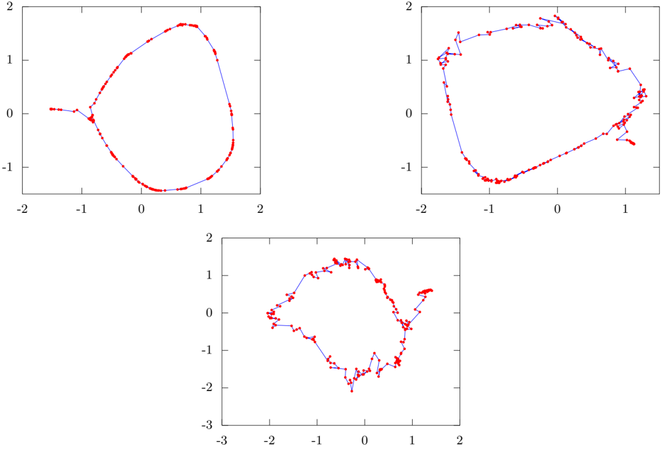
The data consists of a 3-dimensional point cloud of the location of 34 points from a subject performing a run. This leads to a 102 dimensional data set containing 55 frames of motion capture. The subject begins the motion from stationary and takes approximately three strides of run. We hope to see this structure in the visualization: a starting position followed by a series of loops. The data was made available by Ohio State University. The data is characterized by a cyclic pattern during the strides of run. However, the angle of inclination during the run changes so there are slight differences for each cycle. The data is very low noise, as the motion capture rig is designed to extract the point locations of the subject to a high precision.

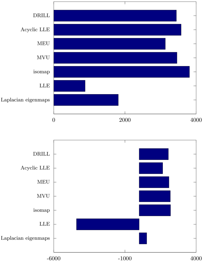
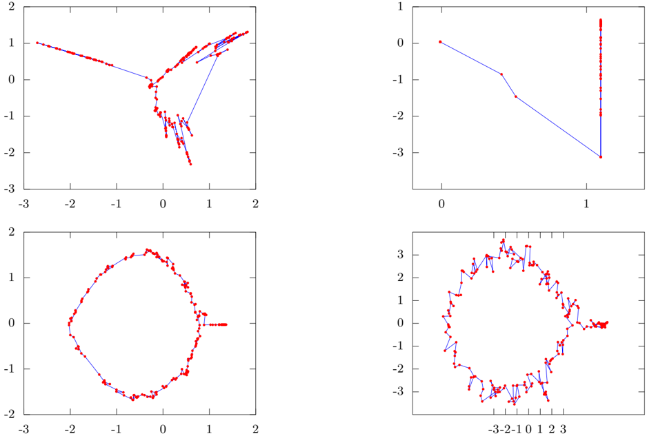
The two dominant eigenvectors are visualized in figure 3-4 and the quality of the visualizations under the GP-LVM likelihood is given in figure 7(a).

There is a clear difference in quality between the methods that constrain local distances (ALLE, MVU, isomap, MEU and DRILL) which are much better under the score than those that don't (Laplacian eigenmaps and LLE). Amongst the distance preserving methods isomap is the best performer under the GPLVM score, followed by ALLE, MVU, DRILL and MEU. The MEU model here preserves the positive definiteness of the covariance by constraining the Lagrange multipliers to be positive (an 'attractive' network as discussed in Section 2.5.1). It may be that this departure from the true maximum entropy framework explains its relatively poorer performance..

4.2 Robot Navigation Example

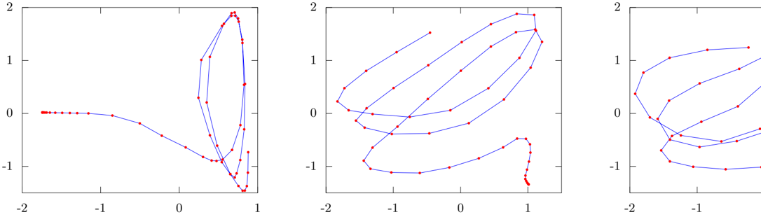
The second data set we use is a series of recordings from a robot as it traces a square path in a building. The robot records the strength of WiFi signals in an attempt to localize its position [see Ferris et al., 2007, for an application]. Since the robot moves only in two dimensions, the inherent dimensionality of the data should be two: the reduced dimensional space should reflect the robot's movement. The WiFi signals are noisier than the motion capture data, so it makes an interesting contrast. The robot completes a single circuit after entering from a separate corridor, so it is expected to exhibit 'loop closure' in the resulting map. The data consists of 215 frames of measurement, each frame consists of the WiFi signal strength of 30 access points.

The results for the range of spectral approaches are shown in figure 5-6 with the quality of the methods scored in figure 7(b). Both in the visualizations and in the GP-LVM scores we see a clear difference in quality for the methods that preserve local distances (i.e. again isomap, ALLE, MVU, MEU and DRILL are better than LLE and Laplacian eigenmaps). Amongst the methods that do preserve local distance relationships MEU seems to smooth the robot path more than the other three approaches. Given that it has the lowest score of the four distance

preserving techniques this smoothing may be unwarranted. MVU appears to have an overly noisy representation of the path.

4.3 Learning the Neighborhood

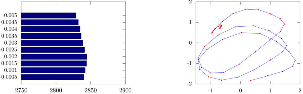
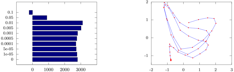
Our final experiments test the ability of L1 regularization of the random field to learn the neighborhood. We firstly considered the motion capture data and used the DRILL with a large neighborhood size of 20 and L1 regularization on the parameters. As we varied the regularization coefficient we found a maximum under the GP-LVM score (figure 8(a)). The visualization associated with this maximum is shown in figure 8(b) this may be compared with figure 4(c) which used 6 neighbors. Finally we investigated whether L1 regularization alone could recover a reasonable representation of the data. We again considered the motion capture data but initialized all points as neighbors. We then applied L1 regularization to learn a neighborhood structure. Again a maximum under the GP-LVM score was found (figure 9(a)) and the visualization associated with this maximum is shown figure 9(b).

The structural learning prior was able to improve the model fitted with 20 neighbors considerably until its performance was similar to that of the the six neighbor model shown in figure 4(c). However, L1 regularization alone was not able to obtain such a good performance, and was unable to tease out the starting position from the rest of the run in the final visualization. It appears that structural learning using L1-priors for sparsity is not on its own enough to find an appropriate neighborhood structure for this data set.

5 Discussion and Conclusions

We have introduced a new perspective on dimensionality reduction algorithms based around maximum entropy. Our starting point was the maximum variance unfolding and our end point was a novel approach to dimensionality

reduction based on Gaussian random fields and lasso based structure learning. We hope that this new perspective on dimensionality reduction will encourage new strands of research at the interface between these areas.

One feature that stands out from our unifying perspective [see also Ham et al., 2004, Bengio et al., 2004b,a] is the three separate stages used in existing spectral dimensionality algorithms.

1. A neighborhood between data points is selected. Normally k -nearest neighbors or similar algorithms are used.
2. Interpoint distances between neighbors are fed to the algorithms which provide a similarity matrix. The way the entries in the similarity matrix are computed is the main difference between the different algorithms.
3. The relationship between points in the similarity matrix is visualized using the eigenvectors of the similarity matrix.

Our unifying perspective shows that actually each of these steps is somewhat orthogonal. The neighborhood relations need not come from nearest neighbors, we can use structural learning algorithms such as that suggested in DRILL to learn the interpoint structure. The main difference between the different approaches to spectral dimensionality reduction is how the entries of the similarity matrix are determined. Maximum variance unfolding looks to maximize the trace under the distance constraints from the neighbours. Our new algorithms maximize the entropy or, equivalently, the likelihood of the data. Locally linear embedding maximizes an approximation to our likelihood. Laplacian eigenmaps parameterize the inverse similarity through appealing to physical analogies. Finally, isomap uses shortest path algorithms to compute interpoint distances and centres the resulting matrix to give the similarities.

The final step of the algorithm attempts to visualize the similarity matrices using their eigenvectors. However, it simply makes use of one possible objective function to perform this visualization. Considering that underlying the similarity matrix, K , is a sparse Laplacian matrix, L , which represents a Gaussian-Markov random field, we can see this final step as visualizing that random field. There are many potential ways to visualize that field and the eigenvectors of the precision is just one of them. In fact, there is an entire field of graph visualization proposing different approaches to visualizing such graphs. However, we could even choose not to visualize the resulting graph. It may be that the structure of the graph is of interest in itself. Work in human cognition by Kemp and Tenenbaum [2008] has sought to fit Gaussian graphical models to data in natural structures such as trees, chains and rings. Visualization of such graphs through reduced dimensional spaces is only likely to be appropriate in some cases, for example planar structures. For this model only the first two steps are necessary.

One advantage to conflating the three steps we've identified is the possibility to speed up the complete algorithm. For example, conflating the second and third step allows us to speed up algorithms through never explicitly computing the similarity matrix. Using the fact that the principal eigenvectors of the similarity are the minor eigenvalues of the Laplacian and exploiting fast eigensolvers that act on sparse matrices very large data sets can be addressed. However, we still can understand the algorithm from the unifying perspective while exploiting the computational advantages offered by this neat shortcut.

5.1 Gaussian Process Latent Variable Models

Finally, there are similarities between maximum entropy unfolding and the Gaussian process latent variable model (GP-LVM). Both specify a Gaussian density over the training data and in practise the GP-LVM normally makes an assumption of independence across the features. In the GP-LVM a Gaussian process is defined that maps from the latent space, X , to the data space, Y . The resulting likelihood is then optimized with respect to the latent points, X . Maximum entropy unfolding leads to a Gauss Markov Random field, where the conditional dependencies are between neighbors. In one dimension, a Gauss Markov random field can easily be specified by a Gaussian process through appropriate covariance functions. The Ornstein-Uhlbeck covariance function is the unique covariance function for a stationary Gauss Markov process. If such a covariance was defined in a GP-LVM with a one dimensional latent space

then the inverse covariance will be sparse with only the nearest neighbors in the one dimensional latent space connected. The elements of the inverse covariance would be dependent on the distance between the two latent points, which in the GP-LVM is optimized as part of the training procedure. The resulting model is strikingly similar to the MEU model, but in the GP-LVM the neighborhood is learnt by the model (through optimization of X ), rather than being specified in advance. The visualization is given directly by the resulting X . There is no secondary step of performing an eigendecomposition to recover the point positions. For larger latent dimensions and different neighborhood sizes, the exact correspondence is harder to establish: Gaussian processes are defined on

a continuous space and the Markov property we exploit in MEU arises from discrete relations. But the models are still similar in that they proscribe a Gaussian covariance across the data points which is derived from the spatial relationships between the points.

Notes

The plots in this document were generated using MATweave. Code was Octave version 3.2.3 x86_64-pc-linux-gnu

Acknowledgements

Conversations with John Kent, Chris Williams, Brenden Lake, Joshua Tenenbaum and John Lafferty have influenced the thinking in this paper.

References

• Onureena Banerjee, Laurent El Ghaoui, and Alexandre d'Aspremont. Model selection through sparse maximum likelihood estimation for multivariate Gaussian or binary data. Journal of Machine Learning Research , 2007.
• Mikhail Belkin and Partha Niyogi. Laplacian eigenmaps for dimensionality reduction and data representation. Neural Computation , 15(6):1373-1396, 2003. doi: 10.1162/089976603321780317.
• Yoshua Bengio, Olivier Delalleau, Jean-Francois Palement, Nicolas Le Roux, Marie Ouimet, and Pascal Vincent. Learning eigenfunctions links spectral embedding and kernel PCA. Neural Computation , 16(10):2197-2219, 2004a.
• Yoshua Bengio, Jean-Francois Paiement, Pascal Vincent, Olivier Delalleau, Nicolas Le Roux, and Marie Ouimet. Out-of-sample extensions for LLE, isomap, MDS, eigenmaps, and spectral clustering. In Thrun et al. [2004], pages 177-184.
• Julian Besag. Statistical analysis of non-lattice data. The Statistician , 24(3):179-195, 1975.
• George E. P. Box and Norman R. Draper. Empirical Model-Building and Response Surfaces . John Wiley and Sons, 1987. ISBN 0471810339.
• Brian D. Ferris, Dieter Fox, and Neil D. Lawrence. WiFi-SLAM using Gaussian process latent variable models. In Manuela M. Veloso, editor, Proceedings of the 20th International Joint Conference on Artificial Intelligence (IJCAI 2007) , pages 2480-2485, 2007.
• Jerome Friedman, Trevor Hastie, and Robert Tibshirani. Sparse inverse covariance estimation with the graphical lasso. Biostatistics , 9(3):432-441, Jul 2008. doi: 10.1093/biostatistics/kxm045.
• Russell Greiner and Dale Schuurmans, editors. Proceedings of the International Conference in Machine Learning , volume 21, 2004. Omnipress.
• Jihun Ham, Daniel D. Lee, Sebastian Mika, and Bernhard Sch¨ olkopf. A kernel view of dimensionality reduction of manifolds. In Greiner and Schuurmans [2004].
• John M. Hammersley and Peter Clifford. Markov fields on finite graphs and lattices. Technical report, 1971. URL http://www.statslab.cam.ac.uk/ ~ grg/books/hammfest/hamm-cliff.pdf .
• Stefan Harmeling. Exploring model selection techniques for nonlinear dimensionality reduction. Technical Report EDI-INF-RR-0960, University of Edinburgh, 2007.
• Trevor Hastie, Robert Tibshirani, and Jerome Friedman. The Elements of Statistical Learning . Springer-Verlag, 2nd edition, 2009.
• Edwin T. Jaynes. Bayesian methods: General background. In J. H. Justice, editor, Maximum Entropy and Bayesian Methods in Applied Statistics , pages 1-25. Cambridge University Press, 1986.
• Charles Kemp and Joshua B. Tenenbaum. The discovery of structural form. Proc. Natl. Acad. Sci. USA , 105(31), 2008.

• Daphne Koller and Nir Friedman. Probabilistic Graphical Models: Principles and Techniques . MIT Press, 2009. ISBN 978-0-262-01319-2.
• Solomon Kullback and Richard A. Leibler. On information and sufficiency. Annals of Mathematical Statistics , 22: 79-86, 1951.
• Neil D. Lawrence. Gaussian process models for visualisation of high dimensional data. In Thrun et al. [2004], pages 329-336.
• Neil D. Lawrence. Probabilistic non-linear principal component analysis with Gaussian process latent variable models. Journal of Machine Learning Research , 6:1783-1816, 11 2005.
• Kantilal V. Mardia, John T. Kent, and John M. Bibby. Multivariate analysis . Academic Press, London, 1979. ISBN 0-12-471252-5.
• Sam T. Roweis and Lawrence K. Saul. Nonlinear dimensionality reduction by locally linear embedding. Science , 290(5500):2323-2326, 2000. doi: 10.1126/science.290.5500.2323.
• Bernhard Sch¨ olkopf, Alexander Smola, and Klaus-Robert M¨ uller. Nonlinear component analysis as a kernel eigenvalue problem. Neural Computation , 10:1299-1319, 1998. doi: 10.1162/089976698300017467.
• Joshua B. Tenenbaum, Virginia de Silva, and John C. Langford. A global geometric framework for nonlinear dimensionality reduction. Science , 290(5500):2319-2323, 2000. doi: 10.1126/science.290.5500.2319.
• Sebastian Thrun, Lawrence Saul, and Bernhard Sch¨ olkopf, editors. Advances in Neural Information Processing Systems , volume 16, Cambridge, MA, 2004. MIT Press.
• Michael E. Tipping and Christopher M. Bishop. Probabilistic principal component analysis. Journal of the Royal Statistical Society, B , 6(3):611-622, 1999. doi: doi:10.1111/1467-9868.00196.
• Larry A. Wasserman. All of Statistics . Springer-Verlag, New York, 2003. ISBN 9780387402727.
• Kilian Q. Weinberger, Fei Sha, and Lawrence K. Saul. Learning a kernel matrix for nonlinear dimensionality reduction. In Greiner and Schuurmans [2004], pages 839-846.
• Christopher K. I. Williams. On a connection between kernel PCA and metric multidimensional scaling. In Todd K. Leen, Thomas G. Dietterich, and Volker Tresp, editors, Advances in Neural Information Processing Systems , volume 13, pages 675-681, Cambridge, MA, 2001. MIT Press.
• Xiaojin Zhu, John Lafferty, and Zoubin Ghahramani. Semi-supervised learning: From Gaussian fields to Gaussian processes. Technical Report CMU-CS-03-175, Carnegie Mellon University, 2003.