Action Networks: A Framework for Reasoning about Actions and Change under Uncertainty

Adnan Darwiche and Moises Goldszmidt Rockwell Science Center 444 High Street, Suite 400 Palo Alto, CA 94301, U.S.A. { darwiche, moises }<Orpal.rockwell.com

Abstract

This work proposes action networks as a se­ mantically well founded framework for rea­ soning about actions and change under un­ certainty. Action networks add two primi­ tives to probabilistic causal networks: con­ trollable variables and persistent variables. Controllable variables allow the representa­ tion of actions as directly setting the value of specific events in the domain, subject to preconditions. Persistent variables provide a canonical model of persistence according to which both the state of a variable and the causal mechanism dictating its value persist over time unless intervened upon by an ac­ tion (or its consequences). Action networks also allow different methods for quantifying the uncertainty in causal relationships, which go beyond traditional probabilistic quantifi­ cation. This paper describes both recent re­ sults and work in progress.

1 Introduction

The work reported in this paper is part of a project that proposes a decision support tool for plan simu­ lation and analysis. The objective is to assist a hu­ man/ computer planner in analyzing plan trade-offs and in assessing properties such as r e l i a bil i t y , robust­ ness, and ramifications under uncertain conditions. The core of this tool is a framework for reasoning about actions under uncertainty, called action networks. Ac­ tion networks add two primitives to probabilistic causal networks (Bayes networks [12]): controllable variables and persistent variables. Controllable vari­ ables are the building blocks for the representation of actions in the domain. Persistent variables allow the modeling of time and change under uncertain condi­ tions.

Controllable variables can be influenced directly by an agent. Thus, their value can be "set" regardless of the state and influences of a c t ua l possible causes in the domain. In this respect action networks follow the proposal in [8, 5] except for the introduction of the associated notion of a precondition for the action. Ac­ tions will be subject to preconditions connecting con­ trollable variables to other variables that establish con­ ditions for controllability.

At the heart of reasoning about actions lies the issue of modeling persistence and change: how and under what conditions should variables in a given domain persist over time when they are not influenced by ac­ tions? We propose a canonical model for persistence to dictate the states of special variables called persis­ tent variables. Traditionally, the modeling of persis­ tence has been accomplished by relating the state of a variable at time t to its state at previous time-points. Problems with this approach has recently prompted researchers to explicitly model the causal mechanisms between variables in a network, and furthermore to persist the state of this mechanism over time (see Sec­ tion 2.2). In this paper we further develop this model and propose a canonical model for the causal mech­ anisms. This model, called the suppressor model, is based on viewing a non-deterministic causal network as a parsimonious encoding of a more elaborate de­ terministic one in which suppressors (exceptions) of causal influences are explicated, and where all the un­ certainty is in the state of the suppressors. The basic intuition here is that suppressors are believed to per­ sist over time, 1 and that variables tend to persist when causal influences on them are deactivated by these sup­ pressors.

Action networks employ quantified causal structures in the form of networks as a compact specification of a state of belief and as a formal language for specifying changes in a state of belief due to both observations and actions (12, 8, 5]. The causal structure allows us to deal with some of the key obstacles in reasoning about action and change such as, the frame and the concurrency problems, and reasoning about the indi­ rect consequences of actions. To allow for different quantifications of the uncertainty in the causal rela-

1The uncertainty of this persistence is determined by

the specific domain.

tions, an action network will consist of two parts: a directed graph representing a "blueprint" of the causal relationships in the domain and a quantification of these relationships. The quantification introduces a representation of the uncertainty in the domain be­ cause it specifies the degree to which causes will bring about their effects. Action networks will allow un­ certainty to be specified at different levels of abstrac­ tion: point probabilities, which is the common practice in causal networks [12], order-of-magnitude probabil­ ities, also known as c-probabilities [8], and symbolic arguments, which allow one to explicate logically the conditions under which causes would bring about their effects (2]. In this paper, we will concentrate on order­ of-magnitude probabilities as proposed in [8]. Other quantifications are described elsewhere [2, 5].

This paper is organized as follows. Section 2 de­ scribes action networks. It starts with a brief review of network-based representations (Section 2.1), and con­ tinues with a description of the models of time and persistence (Section 2.2). Section 2.3 introduces the suppressor model. The representation of actions can be found in Section 2.4. Finally, Section 3 summarizes the main results and describes future work.

2 Action Networks

The specification of an action network requires three components: (1) the causal relations in the domain with a quantification of the uncertainty in these rela­ tions, (2) the set of variables that are "directly" con­ trollable by actions with the variables that constitute their respective preconditions, and (3) variables that persist over time, which we will call persistences in this paper, and variables that do not persist over time, which we will call events.

Once the domain is modeled using this network-based representation (including uncertainty), an action net­ work will be unfolded to create a more elaborate tem­ poral network that includes additional nodes for repre­ senting actions and for representing the values of vari­ ables at different time points.

In this paper, variables will be denoted by lowercase letters e. Binary variables will be assumed to take val­ ues from {false, tr ue } , which will be denoted by e­ and e+, respectively. For clarity of exposition, vari­ ables will be assumed to be binary, unless stated oth­ erwise, and will be referred to as propositions. An instantiated proposition (or set of propositions) will be denoted by e, and -,e denotes the "negated" value of e.

2.1 Network Representations

We briefly review some of the key concepts behind causal networks in this section given the central role they play in action networks. A causal network con­ sists of a directed-acyclic graph r and a quantification

Table 1: x:-Quantification for the engine_ running f a m ­ ily. It represents the default causal rule "If t u rn _ k e y then engine_ runnin g ".

turn_key	engine_rtmning +	engine_nmning
true	0	2
false	0	0

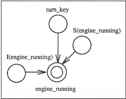
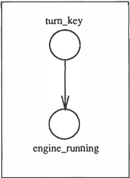
Q over r. Nodes in r correspond to domain variables, and the directed edges correspond to the causal re­ lations among these variables. We denote the set of parents of a node e in a belief network by 1r( e ) . i( e) will denote a state of the propositions that constitute the parent set of e. The set conformed bye and its par­ ents i( e) is usually referred to as the causal family of e. Figure 1 depicts the causal family of engine_running. This network in conjunction with its quantification in terms of the ��:-calculus depicted in Table 1 represents the belief that the engine will be running given that we turn the ignition key.2

The quantification of r over the families in the net­ work encodes the uncertainty in the causal influences between 1r( e) and e. In Bayesian networks, this uncer­ tainty is encoded using numerical probabilities [12]. There are, however, other ways to encode this uncer­ tainty that do not require an exact and complete prob­ ability distribution. Two recent approaches are the ��:-calculus where uncertainty is represented in terms of plain beliefs and degrees of surprise [8], and argu­ ment calculus where uncertainty is represented using logical sentences as arguments [2]. These approaches are regarded as abstractions of probability theory since they retain the main properties of probability includ­ ing Bayesian conditioning [4, 9).

2 Appendix A reviews the main ideas behind the K­ calculus.

An important property of these networks is that a com­ plete and coherent state of belief can be reconstructed from the local quantifications of the families. Thus, they constitute a compact specification of a state of belief. In probabilities for example, given a network containing nodes Xt, ... , Xn,

Similar equations can be obtained for the ��:-calculus and for argument calculus. Since, in this paper we concentrate on a quantification based on plain beliefs using kappa rankings, we provide a brief review of their main properties in Appendix A.

2.2 Time and Persistence

When unfolding a persistent variable in an action net­ work, new variables are added to represent its values at different time points. This leads to a more elaborate causal network that spans over time. The structure of this temporal network is the focus of this section.

Action networks appeal to two assumptions, the re­ alization of which lead to a specific proposal of how to expand an action network into a temporal causal network. The first assumption states that the causal relations between variables at a specific time point are similar to those explicated in the action network. That is, if e has causes c1, ... , Cn in the action network, it will have these causes at every time point. The sec­ ond assumption in action networks relates to temporal persistence. It says that the state of the system mod­ eled by an action network persists over time (with a certain degree of uncertainty) in the absence of exter­ nal intervention. In the remainder of this section we formalize a proposal that realizes these assumptions.

Before we present our persistence model though, it will be illustrative to discuss two intermediate proposals that have inspired the current one.

Persisting Variable States

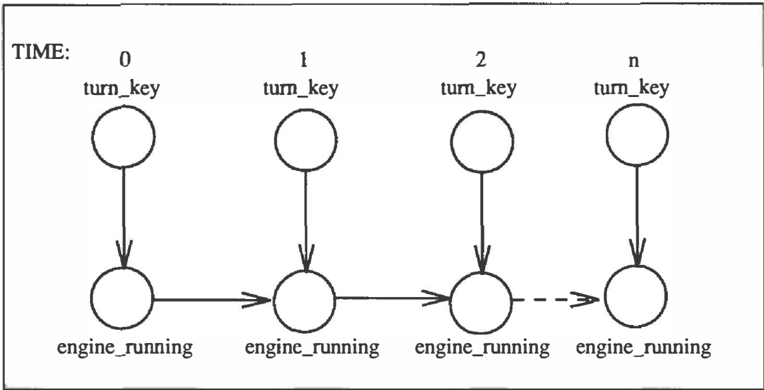
Our first approach required that we make each persis­ tence at timet a direct cause of itself at timet+ 1. This was intended to represent the influence that the past state of a persistence has on its immediate future state. For example, assuming that turn_key is an event and engine_running is a persistence, this proposal leads to Figure 2. This approach is reminiscent of a number of proposals in the literature [13, 6). It fails, however, to capture the notion of persistence that we are after be­ cause it leads to conclusions that are weaker than one would expect. For example, assume that the probabil­ ity of engine_running + at time t given turn_key + at time t and engine_running-at t -1 is .9. Suppose now that we turn the key at time 0 but the engine does not start. We repeat the experiment at times 1, .. . , n1 with similar results (i.e., the engine does not run). In this model of persistence, the probability of engine_running + at time n is still .9 given turn_key + at time n. Yet, intuitively, we would expect the car not to start at time n given the previous sequence of observations.3

Persisting Causal Mechanisms

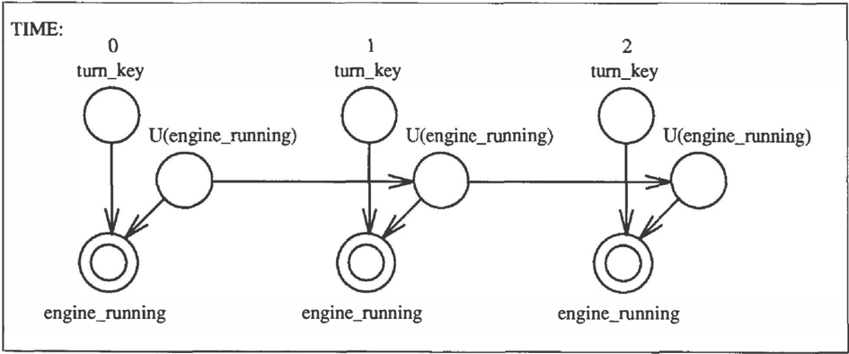
The previous example suggests that it is not enough to persist the state of engine_running. One must also persist the causal mechanism between turn_key and engine_running [11]. The reason why we expect the car not to start is due to our previous observations which lead us to conclude that the causal mechanism between turn_key and engine_running is not behav­ ing normally. Moreover, we seem to assume that the state of the existing mechanism persists over time since no one intervened to change it. One way to capture these intuitions is to explicitly provide a representa­ tion of the causal mechanism between an event e and its causes 1r ( e) in the network. This solution requires that we add (at least) another parent U(e) to each fam­ ily, which represents all possible causal mechanisms between 1r ( e ) and e. The node e will then be deter­ ministic since its state will functionally depend on the state of 1r(e) and U(e). This model is intuitively ap­ pealing in that it encodes the causal relation of a family as a set of functions between the direct causes 1r ( e ) and their effect e, where the state U( e) selects the "active" function that specifies the current causal relation. The likelihood that any of these functions is active depends on the likelihood of the state of the variable U(e).4

Using this approach we persist the functional mecha­ nism represented by the U ( e ) nodes in each family, as shown in Figure 3 with regards to the engine_running family.5

3 This problem will re-appear even if more refined mod­ els of the domain are proposed. One could, for example, add more causal parents representing the exceptions that would prevent the engine from running given that the key is turned. One such exception can be a dead_battery. A l ­ though a step in the right direction, such refinements will not solve the problem above, since we can always repro­ duce the counter-example by introdu6ng the appropriate set of observations (e.g., the battery was OK at each point in time, including time n ) .

tThe assumption behind this representation is that the uncertainty recorded in the quantification of each family in a network r expresses the incompleteness of our knowl­ edge in the causal relation between e and its set of direct causes 1r(e). This incompleteness arises because e inter­ acts with its environment in a complex manner, and this interaction usually involves factors which are exogenous to 1r( e). Furthermore, these factors are usually unknown, un­ observable or too many to enumerate. Thus, we can view a. non-deterministic causal family as a parsimonious repre­ sentation of a. more elaborate, deterministic causal family, where the quantification summarizes the influence of other factors on e.

5Similar representations were used by Pearl and Verma (14] for discovering causal relationships from ob­ servations, and by Druzdzel and Simon (7] in their study about the representation of causality in Bayes networks.

Unfortunately, even though the model in Figure 3 ex­ plicates and persists the causal mechanism between causes and their effects, it is too weak to capture the notion of persistence we are after. Suppose for exam­ ple that we turn the key at time 0. The system will then infer that the engine will be running at time 0 with probability .9. However, the model will not be able to conclude that the engine will continue to be running at times 1, 2, . . . , and so on. In fact, from the topology of Figure 3, we can see that whether the engine is running at time t + 1 is marginally indepen­ dent of whether the key was turned at time t, which is contrary to what we would expect from the persistence assumption.

Persisting Variable States and Causal Mecha­ nisms

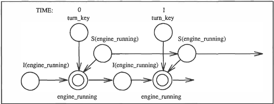
The approach we adopt, depicted in Figure 5, can be regarded as a combination of the temporal net­ works in Figures 2 and 3. The proposition en­ gine_running is functionally determined by turn_key, S( engine_running ) , and I ( engine_running ) . The vari­ able S( engine_ running) captures all possible sup­ pressors of the causal influences that the proposi­ tion turn_key has on engine_running. The variable I( engine_running) decides the state of engine_ running when the the suppressors manage to deactivate the causal influence of turn_key on engine_running, and it is directly influenced by the past state of en-. . gme_runnmg.

In the static case, when time is not involved, the pro­ posal can be viewed as splitting the variable U(e) into two variables, S(e) and /(e). Note, however, that once we expand over time the notion of a causal mecha­ nism has a broader scope because it has to account for the previous value of proposition e. The semantics of the variable S( e ) assumes that the uncertainty in the causal relation between e and its causes 1r( e) is due to a set of abnormalities and exceptions that suppress this causal influence. When this influence is suppressed due to these exceptions and abnormalities the value of e is set according to its previous state (represented by the variable I (e)). This model of persistence makes two assumptions. First, it assumes that the state of suppressors tend to persist over time (with a degree of uncertainty determined by the specific application). Second, it assumes that the state of variable/( e) is de­ termined by the state of e at the previous time point. 6

This model is not only intuitive and solves the prob­ lems outlined above, but it allows for a modular quan­ tification of the network: the uncertainty in the causal relations, the uncertainty in the persistence of suppres­ sors, and the uncertainty in the persistence of variables

An expansion similar to the one in Figure 3 is used by Balke and Pearl [1] for answering probabilistic counter­ factual queries, and by H ec k er ma n and Shachter [11] for capturing the notion of causal persistence.

6Both these assumptions can be relaxed and lead to more elaborate models (see S ec ti o n 3).

can be specified independently (see Eqs. 5 and 6).

The following section will discuss the suppressor model in more detail.

2.3 The Suppressor Model

To formally describe the suppressor model we first ex­ amine how it expands a "static" causal network into a functional one, where all causal relations are determin­ istic and all the uncertainty is about the states of root nodes. Then we show how this functional expansion of a causal network lends itself naturally for captur­ ing the persistence assumptions that we stated in the previous section.

As a proposal for functionally expanding a causal net­ work, the suppressor model is based on the following intuition. The uncertainty in the causal influences be­ tween 1r( e) and e is a summary of the set of excep­ tions that attempt to defeat or suppress this relation. For example, "a banana in the tailpipe" is a possible suppressor of the causal influence that turn_key has on engine_running. The expansion into the suppres­ sor model makes the uncertain causal relation between 1r( e ) and e functional by adding a new parent S( e ) to the family, which corresponds to the suppressors to the causal relation. In addition to S( e), another par­ ent /(e) is added, which will set the state of e in those cases in which the suppressors manage to defeat the causal influence of 7!'( e ) on e. In these cases we say that the suppressors are "active" . Figure 4 depicts the expansion of the engine_running family.

Once a causal network is functionally expanded ac­ cording to the suppressor model, the persistence as­ sumption stated in the previous section can be for­ malized by taking the variable /(e) to represent the previous state of e -see Figure 5. The intuition be­ ing that in those cases where the suppressors manage to prevent the natural causal influences on e, the state

of e should simply persist and follow its previous state.

We will now present the suppressor model formally. Let S(e) take values out of the set {w0,w1,w2, . . . )1 w h e r e S( e) = ws stands for "a sup � ressor o � stre ? gth s is active." The fu nc t i o n F relatmg e to 1ts duect causes 1r ( e ) , the suppressors S( e), and the variable /(e) is given by

Where ��: ( e J7r( e )) represents the strength of belief in th . e causal relation between 1r(e) and e. Eq. �says that tf the strength of the active suppressor w' is less than the causal influence of 1r( e) on e, then the state of e is dictated by the causal influence. Otherwise, the sup­ pressor is successful, t he causal influence is suppressed, and the state of e is the same as the state of I (e).

The translation ofF into a K matrix is given by below:

The prior distribution of beliefs on S( e) is given by

which reflects the intuition that suppressors are typi­ cally inactive, and that the stronger the suppressor is, the more unlikely that it will be active.

Using the suppressor model, we can take any n o n ­ deterministic network quantified with kappas and au­ tomatically expand it into a functional network in the

7In general, the suppressor takes values in {w0, w1, w2, · · . , w00 }. In practice, however, it suffices for the suppressor to take values in { wk} where the ranking k appears in the matrix of e.

sense that all causal relations are deterministic and the only uncertainty is re g a r d i ng suppressors. Moreover, we get the f o l l o w in g guarantee about the r es u lti ng functional n e t wo rk , which says that the new network captures all the information which the initial network was set to capture. L e t K represent the quantification of a non-deterministic network and let 1\.1 represent the quantification of its functional expansion:

The proof of this theorem relies on m a rg ina li z i n g K'(CJi(e), S(e), f(e)) over all the states of S(e) and I( e).

Table 2 shows the automatic functional expansion of the causal relation between engine_running a n d 1r( engine_running) (depicted in Figure 1 and K­ q u a n t i fi ed in Table 1) reflecting Eq. 2.

Table 2: Deterministic function relating en­ gine.running and its parents in the suppressor model.

turn-k�y	S en gin�....runnin�	I enJ{ine-runnin�r	eriiine_runnans
uue	..,u	true	true
uue	..,u	fa.Jse	true
&rue	w/.	&rue	true
uue	w•	fa.he	false
false	..,v	true	fru.e
fa.l:;e	..,v	fa..lse	r .. lae
false	w•	true	true
faJ�e	w"	false	fa.be

In order to complete the temporal expansion, shown in Figure 5, we must quantify the uncertainty on the persistence arcs. Causal families are connected, across time points, through the I (e) node and the suppressor S(e) node. The conditional beliefs k(S(et+z)JS(et)) and K(f(e1+t)Jej) wi l l formally determine the strength of persistence across time. Both conditional beliefs will encode a bias against a change of state, which captures

the intuition that any change of state must be causally motivated. Note that this quantification is done mod­ ularly and independently of the quantification of the uncertainty in the causal relations. This separation is important for fast and efficient model building.

The quantification of these beliefs will be of course tied directly with an actual application and a specific domain. In our experiments, and for the planning do­ main implemented we had intuitive results with the following model in which the strength of the persis­ tence assumption is proportional to the strength of the change in the state of the suppressor:

The assumption of persistence for the I ( e ) node cor­ responds to the following equation:

Since I( et ) determines the state of et+l when suppres­ sors are active, the number p can be interpreted as the degree of surprise in a non-causal change of state of the proposition et+l·s

Example. Consider the engine_running network in Figure 1 quantified as in Table 1. Assume that this network is temporally expanded using the suppressor model (see Eq. 3 and Figure 5). Given the ignition key is turned at times 1, 2, 3, . . . , n1 and that the engine is not running at times 1, 2, 3, . . . , n -1, the model will yield the belief that the engine will not be running at time n, given that the key is turned at time n. On the other hand, given that the key is turned at time 0, the system will infer that the engine will be running at time 0, and moreover that it will be running at times 1, ... , n.

2.4 Actions and Preconditions

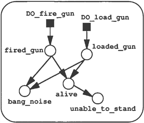
For the representation of actions, we essentially follow the proposal in [8], which treats actions as external di­ rect interventions that deterministically set the value of a given proposition in the domain. Actions are spec­ ified by indicating which nodes in the causal network are controllable and under what preconditions. Syn­ tactically, we introduce a new node " I" denoting controllability. In Figure 6 for example, both fired_gun and /oaded_gun are controllable propositions. A suit­ able precondition for both nodes can be holding_gun, which can be represented as just another direct cause of these nodes. The corresponding matrices will then be constructed to reflect the intuition that the action doe will be effective only if the precondition is true; otherwise, the state of a node e is decided completely by the state of its natural causes (that is, excluding doe and the preconditions of do,). Let the variable doe take the same values as e in addition to the value

8This value does not need to be constant, although it will assumed to be so in the remainder of the paper.

idle.9 The new parent set of e after e is declared as controllable will be 1r( e) U {doe}. The new ranking ��:'(fli(e) 1\ d�e) is

For simplicity of exposition we have omitted possible preconditions. Their inclusion will just involve a re­ finement of the cases in Eq. 7 to reflect the fact that an action is possible iff its preconditions are satisfied.

The advantage of using this proposal as opposed to others, such as STRIPS, is that the approach based on direct intervention takes advantage of the network rep­ resentation for dealing with the indirect consequences of actions and the related frame problem. In specify­ ing the action "shooting", for example, the user need not worry about how this action will affect the state of other related consequences such as bang_noise or alive (see Figure 6).

Example. Consider the example in Figure 6 encod­ ing a version of the Yale Shooting Problem (YSP) [10]. The relevant piece of causal knowledge available is that if a victim is shot with a loaded gun, then she/he will die. There are two possible actions, shooting and load­ ing/unloading the gun. It is also assumed that both loaded and alive persist over time. Given this infor­ mation the implementation of action networks will ex­ pand the network in Figure 6 both functionally and temporally.

In the first scenario, we observe at time 0 that the individual is alive and that the gun is loaded, and that

9Thus, ife is binary d�e E {e+,e-, idle}.

there i s a shooting action at time 2. The model will yield that alive at ti m e 2 will be false.10 This scenario shows the interplay between the persistences and the causal influences in the network.

In the second scenario, it is observed that at time 2 alive is t ru e (the victim actually survived the shoot­ ing ) . The model will then conclude that: first, the gun must have been unloaded prior to the shooting (although it i s not capable of asserting when), and fur­ thermore, the belief of an action leading to u nloa d i ng the gun increases (proportional to the degree of per­ sistence in l oa din g ) . This scenario displays the model ca p a bi lit i es for performing abductive reasoning includ­ ing reasoning about the set of actions that would yield a given observation.

3 Conclusions and Future Work

We described the models of time, persistence, and ac­ tion that constitute the c o r e of action networks as a formalism for reasoning about action s and change un­ der uncertainty. The notion of persistence was for­ malized through the suppressor model which evolved from other proposals for exte n di ng causal networks over time. The suppressor model should be viewed as one canonical model for representing persistence. Re­ laxing the assumptions in this m ode l will yield other possible, more complex representations. For exa m p l e we can make the I (e) node depend on more than one past i n st a nc e of e. Th is would al low the representation of time-decaying functions for the dependence of e on its past values. We are c u rren t l y exploring and charac­ t er i z i n g this and other alternatives with the objective to provide a library of such models that would assist the user in encoding the dynamics of causal relations in the d oma i n of interest.

We also intend to add notions of utility and pr ef er e nces on outcomes and to explore the use of action networks in the formulation of a plan, given a set of objectives. The paths we are currently exploring include abduc­ tive m eth o ds for uncovering the sequence of actions that can lead to a specific set if beliefs, and the p os ­ sibility of interfacing action networks as an evaluation component to a planning module.

This paper has focused on the ��:-calculus in st an t ia ­ tion of action networks. Future work includes all ow i n g other quantifications of un c e rta i nt y , such as p rob a b i li ­ ties, and arguments, and even a mixture of these. We are also s tu dyin g a p r o b a b i l i s t i c (and argument-based) interpretation of the suppressor model. The first st e ps toward the quantification of action networks with ar­ guments is reported in [5].

Finally we remark that all the fea t u r e s of action net-

10The reasons for this conclusion are due to the con­ ditional independences assumed in the causal network representation. They are formally explained in depth in [12][Chapter 10] and [8].

works described in this paper, inc ludin g the su p pr es­ sor model expansion, the temporal expansion, and the s p eci fi cati on of actions, are fully i m ple m ente d on top of CNETS [3].U A l l the examples described in this paper were tested u si n g this implementation.

Acknowledgments

We wi sh to thank P. Da g u m for discussions on the na­ ture and p r op ert ie s of t he f un c t io n a l e x p a ns ion of a causal network. We also thank C. Boutilier, J. Pearl, Y. Shoham and the Nobotics group at Stanford for dis­ cussions on the re p re s en tation of actions. D. Draper, D. Etherington, and D. H e c k e r ma n provided useful comments on a previous version of this paper.

This work was p a rtial ly supported by ARPA contract F30602-91-C-0031, a n d by IR&D f un d s from Rockwell Science Center.

A Appendix: A Review of The Kappa Calculus.

We p r o vi d e a b ri e f summary of the ��:-calculus and how it can quantify over the causal relations in a n et w o r k r.

Let M be a set of worlds, each wo rl d m E M being a truth-value assignment to a finite set of atomic propo­ sitional variables (e1, e2, . . . , e0 ) . Thus any world m can be represented by the conjunction of ei /1. .. . /1. e-;;. A belief ranking function ��:(m) is an as si gn men t of non-negative integers to the elements of M such t ha t ��:(m) = 0 fo r at least one m E M. I nt u i tivel y , K(m) represents the degree of s u r p r is e associated with find­ i n g a world m r e a li z e d , worlds assigned 11: = 0 a r e considered serious possibilities, an d w or lds ass i gne d 11: = oo are considered absolute impossibilities. A p r opos i ti o n e is believed iff ��:(...,e) > 0 ( w i th degree k iff ��:(...,e) = k), where

��:(m) can be considered an order-of-magnitude approx­ imation of a probability function P(m) by wr i t i ng P(m) as a polynomial of some small q u a n t i t y t a nd taking the most significant term of that polynomial, i.e., P(m) � Cc:"(m). Treating E as an infinitesi­ mal quantity induces a conditional ranking function ��:(eic) on propositions and wffs governed by p r ope r ti e s derived from the £-probabilistic interpretation [9).

A causal s tr u c t ur e r can b e q ua n tifi e d u si ng a rank­ ing belief function 11: by specifying the conditional be­ lief for each proposition e given every state of i(e), t ha t is ��:( eji( e)). T hu s , for e x amp le , Table 1 shows

11CNETS is an experimental environment for represent­ ing and reasoning with generalized causal networks, which allow the quantification of uncertainty using probabilities, " degrees of belief, and logical arguments [2].

the ��:-quantification of the engine_running family in Figure 1. Table 1 is called the "��:-matrix" for the en­ gine_running family. It represents the default causal rule: "If turn_key + then engine_ running + ".

The ��:-calculus does not require commitment about the belief in e + or e-. Thus, as Table 1 in­ dicates, we may be ignorant about the status of the engine_running given that the ignition key is not turned. In such a case the user may specify that both ��:(engine_running + jturn_key-) = ��: ( engine_running-lturn_key-) = 0 indicating that both alternatives are plausible.

Once similar matrices for each one of the families in a given network r are specified, the complete ranking function can be reconstructed by requiring that

and queries about belief for any proposition and wff can be computed using any of the well-known dis­ tributed algorithms for belief update (12, 3]. The class of ranking functions that comply with the require­ ments of Eq. 9 for a given network rare called stratified rankings. These rankings present analogous properties about conditional independence to those possessed by probability distributions quantifying a network with the same structure (8].

References

• (1] A. Balke and J. Pearl. Probabilistic evaluation of counterfactual queries. In Proceedings of the 101h Conference on Uncertainty in Artificial, Intelli­ gence, 1994. In press.
• A. Darwiche. Argument calculus and networks. In Proceedings of the. Ninth Conference. on Un­ certainty in Artificial Intelligence., pages 420-421, Washington DC, 1993.
• A. Darwiche. CNETS: A computational envi­ ronment for causal networks. Technical memo­ randum, Rockwell International, Palo Alto Labs., 1994.
• A. Darwiche and M. Ginsberg. A symbolic gen­ eralization of probability theory. In Proceedings of the American Association for Artificial Intelli­ gence Conference, pages 622-627, San Jose, CA, 1992.
• A. Darwiche and J. Pearl. Symbolic causal net­ works for reasoning about actions and plans. Working notes: AAAI Spring Symposium on Decision-Theoretic Planning, 1994.
• T. Dean and K. Kanazawa. A model for reasoning about persistence and causation. Computational Intelligence, 5(3): 1442-150, 1989.
• M. Druzdzel and H. Simon. Causality in Bayesian belief networks. In Proceedings of the 9111 Confer­ ence in Uncertainty in Artificial Intelligence Con­ ference, pages 3-11, Washington D.C., 1993.
• M. Goldszmidt and J. Pearl. Rank-based sys­ tems: A simple approach to belief revision, be­ lief update, and reasoning about evidence and ac­ tions. In Principles of Knowledge Representation and Reasoning: Proceedings of the Third Interna­ tional Conference, pages 661-672, Boston, 1992.
• M. Goldszmidt and J. Pearl. Reasoning with qual­ itative probabilities can be tractable. In Proceed­ ings of the 8111 Conference on Uncertainty in AI, pages 112-120, Stanford, 1992.
• S. Hanks and D. McDermott. Non-monotonic logics and temporal projection. Artificial Intel­ ligence, 33:379-412, 1987.
• D. Heckerman and R. Shachter. A timeless view of causality. In Proceedings of the 10111 Conference on Uncertainty in Artificial, Intelligence, 1994. In press.
• J. Pearl. Probabilistic Reasoning in Intelligent Systems: Networks of Plausible Inference. Mor­ gan Kaufmann, San Mateo, CA, 1988.
• J. Pearl. From conditional oughts to qualitative decision theory. In Proceedings of the 9th Confer­ ence on Uncertainty in AI, pages 12-20, Wash­ ington D.C., 1993.
• (14] J. Pearl and T. Verma. A theory fo inferred cau­ sation. In Proceedings of Principles of Knowl­ edge Representation and Reasoning, pages 441452, Cambridge, MA, 1991.