Aggregating Learned Probabilistic Beliefs

Pedrito Maynard-Reid II

Computer Science Department Stanford University Stanford, CA 94305-9010

pedmayn®cs.stanford.edu

Abstract

We consider the task of aggregating beliefs of sev­ eral experts. We assume that these beliefs are rep­ resented as probability distributions. We argue that the evaluation of any aggregation technique depends on the semantic context of this task. We propose a framework, in which we assume that nature generates samples from a 'true' distribution and different experts form their beliefs based on the subsets of the data they have a chance to observe. Naturally, the optimal ag­ gregate distribution would be the one learned from the combined sample sets. Such a formulation leads to a natural way to measure the accuracy of the aggregation mechanism.

We show that the well-known aggregation operator LinOP is ideally suited for that task. We propose a LinOP-based learning algorithm, inspired by the techniques developed for Bayesian learning, which aggregates the experts' distributions represented as Bayesian networks. We show experimentally that this algorithm performs well in practice.

1 Introduction

Belief aggregation of subjective probability distributions has been a subject of great interest in statistics (see [GZ86, CW99]) and, more recently, artificial intelligence (e.g., [PW99]) and machine learning (ensemble learning in par­ ticular [PMGHOO]), especially since probabilistic distribu­ tions are increasingly being used in medicine and other fields to encode knowledge of experts. Unfortunately, many of the aggregation proposals have lacked sufficient semantical underpinnings, typically evaluating a mecha­ nism by how well it satisfies properties justified by little more than intuition. However, as has been noted in other fields such as belief revision (cf. [FH96]), the appropriate­ ness of properties depends on the particular context.

We take a more semantic approach to aggregation: we first describe the realistic framework in which the experts or sources learn their probability distributions from data us­ ing standard probabilistic learning techniques. We assume

Urszula Chajewska

Computer Science Department Stanford University Stanford, CA 94305-9010

[email protected] a Decision Maker (DM)- the traditional name for the ag­ gregator - wants to aggregate a set of these learned dis­ tributions. This framework suggests a natural optimal ag­ gregation mechanism: construct the distribution that would be learned had all the sources' data sets been available to the DM. Since the original data sets are generally not avail­ able, the aggregation mechanism should come as close as possible to reconstructing the data sets and learning from the combined set.

For intuition, consider the the task of creating an expert system for some specialized medical field. We would like to take advantage of the expertise of several doctors work­ ing in this field. Each of these doctors sharpened his knowledge by following many patients. The doctors can no longer recall the specifics of each case, but they have formed over the years fairly accurate models of the do­ main that can be represented as sets of conditional prob­ abilities. (In fact, many expert systems have been created over the years by eliciting such conditional probabilities from experts [HHN92].) Of course, if there was a doctor who had seen all of the patients the others doctors saw, the ideal expert system would result from eliciting her model. However, there isn't one such expert. Therefore, our sys­ tem would benefit from incorporating the knowledge of as many experts as we can find. The system would also ac­ count for the differing levels of experience of different doc­ tors - some of them may have practiced for much longer than others.

One of the best-known aggregation operators is the Lin­ ear Opinion Pool (LinOP) which aggregates a set of distri­ butions by taking their weighted sum. It has been shown in the statistics community that, under some intuitive as­ sumptions, learning the joint distribution from the com­ bined data set is equivalent to using LinOP over the individ­ ual joint distributions learned from the individual data sets. However, whereas the weights in typical uses of LinOP are often criticized for being ad-hoc, our framework pre­ scribes semantically-justified weights: the estimated per­ centages of the data each source saw. Intuitively, a high weight means we believe a source has seen a relatively

二

一

large amount of data and is, hence, likely to be reliable.

However, joint distributions are hardly the preferred rep­ resentation for probabilistic beliefs in real-world domains. BNs (aka belief networks, etc.) [Pea88] have gained much popularity as structured representations of probability dis­ tributions. They allow such distributions to be represented much more compactly, therefore often avoiding exponen­ tial blowup in both memory size and inference complexity.

Thus, we assume the sources beliefs are BNs learned from data. According to our semantics, the aggregate BN should be one the DM would learn from the combined sets of data. We describe a LinOP-based BN aggregation algorithm, in­ spired by the algorithm designed to learn BNs from data. The algorithm uses sources' distributions instead of sam­ ples to search over possible BN structures and parameter settings. It takes advantage of the marginalization prop­ erty of LinOP to make computation more efficient. We ex­ plore the algorithm's behavior by running experiments on the well-known, real-life Alarm network [BSCC89] and on the smaller artificial Asia network [LS88].

2 Formal Preliminaries

We restrict our attention to domains with discrete variables. We consider how to compute the aggregate distribution, and how the accuracy of our computation depends on how much we know about the sources.

Formally, we consider the following setting: There are L sources and N discrete random variables, where each vari­ able X has domain dom(X). We follow the convention of using capital letters to denote variables and lowercase let­ ters to denote their values. Symbols in bold denote sets. W is the set of possible worlds defined by value assignments to variables. The true distribution or model of the world is 1r. Each source i has a data set Di sampled from (unknown to us) rr. We will assume that each Di is finite of size Mi. The corresponding empirical (i.e., frequency) distribution is Pi· Each source i learns a distribution Pi over W. This is i's model of the world. The combined set of samples is D = UiDi of size M. The corresponding empirical distri­ bution is p. The DM constructs an aggregate distribution p. The optimal aggregate distribution p * is posited to be the distribution the DM would learn from D.

Since it is unrealistic to expect the DM to have access to the sources' sample sets, we consider how to use information about the sources' learned distributions to at least approx­ imate p * . Specifically, we consider the situation where the DM knows the sources' distributions and has a good esti­ mate of the percentage ai = Md M of the combined set of samples each source i has observed as well as what learn­ ing method it used.

We make a number of assumptions. First, we assume that the samples are not noisy or otherwise corrupted, and they are complete (no missing values).

Second, we assume that the individual sample sets are dis­ joint (so M = Ei Mi). This implies that the concatenation of the Di equals D, so we don't have to concern ourselves with repeats when aggregating. This assumption is not al­ ways appropriate. It is invalidated when multiple sources observe the same event. However, there are interesting do­ mains where this property holds. For example, in our mo­ tivating medical domain, doctors are likely to have seen disjoint sets of patients.

Third, we assume that the sources believe their samples to be liDindependent and identically distributed. The ma­ chine learning algorithms used in practice commonly rely on this assumption.

Finally, we assume that the samples in the combined set D are sampled from 1r and liD. This assumption may appear overly restrictive at first glance. For one, it may seem to preclude the common situation where sources receive sam­ ples from different subpopulations. For example, if doctors are in different parts of the world, the characteristics of the patients they see will likely be different.

In fact, we can accomodate this situation within our frame­ work by assuming 1r is a distribution over the domain vari­ ables and a source variable S which takes the different sources as values; S = i means source i observed the in­ stantiated domain variables. This generalized distribution is sampled liD. Each Di consists of the subset of samples where S = i. It is not necessary to keep around the S val­ ues; computing the Pi and p * without S will give the same results as learning distributions over the complete samples and marginalizing outS. Thus, although samples will be liD, different subpopulation distributions will be possible, captured by different conditional probability distributions of the domain variables given distinct values of S. 1

3 Aggregating Learned Joint Distributions

We first consider the case where sources have learned joint distributions, and the aggregate is also a joint.

3.1 Learning joint distributions: review

Given samples of a variable X, the goal of a learner is to es­ timate the probability of future occurences of each value of X. In our setting, the domain of X is Wand the parameters that need to be learned are the IWI probabilites. The dis­ tribution over X is parameterized by 0. Two standard ap­ proaches are Maximum Likelihood Estimation (MLE) and Maximum A Posteriori estimation (MAP).

1 Two implications of this formulation are that the assumption that the D; are disjoint is implicit and a; will approach 1r(S = i) as M approaches oo for all i.

An MLE learner chooses the member of a specified family of distributions that maximizes the likelihood of the data:

Definition 1 If X is a random variable, dom(X) = {xJ, ... ,xk}, and0 = (el,····ek) where e i = P(x; I 8), then the MLE distribution over X given data set D is

It is easy to show that the MLE distribution is the empirical distribution if samples are liD.

MAP learning, on the other hand, follows the Bayesian ap­ proach to learning which directs us to put a prior distribu­ tion over the value of any parameter we wish to estimate. We treat these parameters as random variables and define a probability distribution over them. More formally, we now have a joint probability space that includes both the data and the parameters.

Definition 2 If X is a random variable, dom(X) = {x1, ... ,xk}, ande = (eJ, ... ,ek) wheree; = P(x; I 0), then the MAP distribution over X given data set D and prior P(e) is the distribution

The appropriate conjugate prior for variables with multino­ mial distributions is Dirichlet. Dir( e Ill, .. . ' /k), where each li is a hyperparameter such that'"'(; > 0.

We will assume that Dirichlet distributions are assessed us­ ing the method of equivalent samples: given a prior dis­ tribution p over X and an estimated sample size �� '"Yi is simply p(x;)�. We use these to parameterize MAP:

Definition 3 If X is a random variable, dom(X) {xt, ... , xk}, e = (ell . . . , ek) where e; = p(x; I 0), p is a probability distribution over X, and � > 0, then MAP(X, (p, �),D) denotes the distribution MAP(X, po, D) where Po = Dir(0lp(xt)�, ... , p(xk)�).

We will omit the X argument from the MLE and MAP no­ tation since it is understood.

3.2 LinOP: review

Let us tum to the problem of aggregation. We will show that joint aggregation essentially reduces to LinOP. LinOP was proposed by Stone in [Sto61], but is generally at­ tributed to Laplace. It aggregates a set of joint distributions by taking a weighted s u m of them:

Definition 4 Given probability distributions p1, ... , P L and non-negative parameters {31, · . . , {3 L such that Li f3 i = 1, the LinOP operator is defined such that, for anyw E W,

LinOP is popular in practice because of its simplicity. As described in [GZ86], it also has a number of attractive properties such as unanimity (if all the Pi == p', then LinOP returns p'), non-dictatorship (no one input is always followed), and the marginalization property (aggregation and marginalization are commutative operators). However, LinOP has often been dismissed in the aggregation commu­ nities as a normative aggregation mechanism, primarily be­ cause it fails to satisfy a number of other properties deemed to be necessary of any reasonable aggregator, e.g., the ex­ ternal Bayesianity property (aggregation and conditioning should commute) and the preservation of shared indepen­ dences. Furthermore, typical approaches to choosing the weights are often criticized as being ad-hoc.

However, this dismissal may have been overly hasty. LinOP proves to be the operator we are looking for in our framework: using it is equivalent to having the DM Jearn from the combined data set under intuitive a ssum p t i o n s .

3.3 MLE aggregation

Suppose the sources and the DM are MLE learners. As has been known in statistics for some time, the DM need only compute the LinOP of the sources' distributions.

Proposition 1 ([Win68, Mor83]) If Pi = MLE(Di) for each i E {1, .. . ,£} and p * = MLE(D), then p * = LinOP(a1, PI, . . . , aL, PL).

Although straight-forward, this proposition is illuminating. For one, the weight corresponding to each source has a very clear meaning; it is the percentage of total data seen by that source. The DM only needs to provide accurate estimates of these percentages. A high weight indicates that the DM believes a source has seen a relatively large amount of data and is, hence, likely to be very reliable. Thus, we address a common criticism of LinOP, that the weights are often chosen in an ad-hoc fashion. Also, if M is known, the DM can compute the number of samples in D that were w: MLinOP(al,PI, . . . ,aL, pL). Thus, LinOP can be viewed as essentially storing the sufficient statistics for the DM learning problem.

It is now easy to see why a property such as preservation of independence will not always hold given our learning­ based semantics. In our framework, sources do not have strong beliefs about independences; any believed indepen­ denc e depends on how weJl it fits the source's data. The independence preservation property does not take into ac­ count the possibility that, because of limited data, sources may all have learned independences which are not justified if all the data was taken into account.

一

Consider, for example, the following distribution over two variables A and B: w(ab) = 1/4, w(ab) = 1/6, 1r(ab) = 1/3, and 1r(ab) = 1/4. Obviously, A and B are not in­ dependent. Suppose two sources have each received a set of six samples from this distribution: D1 consists of one each of ab and ab, two each of ab and ab; D2 consists of one each of ab and ab, two each of ab and ab. Further suppose each used MLE to learn a distribution over A and B. A and B are independent in each of these distributions. The LinOP distribution, on the other hand, effectively takes into account the evidence seen by both sources and actually computes 1r where the variables are not independent.

3.4 MAP aggregation

MLE learners are known to have problems with overfitting and low-probability events for which data never material­ ized. MAP learning often does a better job of dealing with these problems, especially when data is sparse.

Consequently, suppose the sources and the DM are MAP learners with Dirichlet priors. The optimal aggregate dis­ tribution is a variation on LinOP: 2

Proposition 2 Suppose, for each i E {1, .. . , L }, p; = MAP((p;,0,D;) andp* = MAP((p,�),D;). Then,

The first term in Equation 1 is the OM's MAP estimation, the second term accounts for the sources' priors by sub­ tracting out their effect.

Corollary 2.1 Suppose, for each i E { 1 , ... , L}, Pi = MAP((p;, �;), D;) andp* = MAP((p,�), Di). Then,

Thus, as M becomes large, the LinOP distribution ap­ proaches p*. This is not surprising since it is well-known that MLE learning and MAP learning with Dirichlet priors are asymptotically equivalent. The implication is that if M is large, not only do we not need to know M to aggregate, we do not need to know what priors the sources used ei­ ther. And if we approximate the aggregate distribution by the LinOP distribution, this approximation will improve the more samples seen by the sources.

4 Aggregating Learned Bayesian Networks

Bayesian networks (BNs) are structured representations of probability distributions. A BN b consists of a directed

2We omit proofs for lack of space.

acyclic graph (DAG) g whose nodes are theN random vari­ ables. The parents of a node X are d e n o ted by P a ( X ) ; p a (X) denotes a particular assignment to P a (X) . The structure of the network encodes marginal and conditional independencies present in the distribution. Associated with each node is the conditional probability distribution (CPO) for X given Pa(X).

We consider the case where sources' beliefs are represented as BNs learned from data. We briefly review the tech­ niques used for learning BNs from data. For a more de­ tailed presentation, see [Hec96].

4.1 Learning Bayesian networks: review

If the structure of the network is known, the task reduces to statistical parameter estimation by MLE or MAP. In the case of complete data, the likelihood function for the entire BN conveniently decomposes according to the structure of the network, so we can maximize the likelihood of each parameter independently.

If the structure of the network is not known, we have to ap­ ply Bayesian model selection. More precisely, we define a discrete variable G whose states g correspond to possible models, i.e., possible network structures; we encode our uncertainty about G with the probability distribution P(g). For each model g, we define a continuous vector-valued variable 8g. whose instantiations Bg correspond to the pos­ sible parameters of the model. We encode our uncertainty about 8g with a probability distribution P(Bg I g).

We score the candidate models by evaluating the marginal likelihood of the data set D given the model g, that is, the Bayesian score P(D I g) = J P(D I Bg, g)P(Bg I g)P(g)d8g.

In practice, we often use some approximation to the Bayesian score. The most c ommo n l y used is the MDL score, which converges to the Bayesian score as the data set becomes large. The MDL score is defined as

where Dim(g'] is the number of independent parameters in the graph and DL(g') is the description length of g'. Find­ ing the network structure with the highest score has been shown to be NP-hard in general. Thus, we have to resort to heuristic search. Since the search can easily get stuck in a local maximum, we often add random restarts to the pro­ cess. The BN learning algorithm is presented in Figure 1.

Why are we interested in learning BNs rather than joint

Figure 1: Bayesian network learning algorithm.

1 .	pick a random DAG g
2.	parameterize g to form b
3.	scoreb
4.	loop
5.	for each DAG g' differing from g by adding, removing, or reversing an edge
6.	parameterize g' to form b'
7.	score b'
8.	pick the b' with the highest score and replace g with g' and b with b' if score(b') > score(b)
9.	until no further change g
10.	return b.

distributions? Besides some obvious reasons concerning compact representation and efficient inference, a distribu­ tion learned by the BN algorithm may be closer to the orig­ inal distribution used to generate the data in the first place.

First, note that the networks which can be parameterized to represent exactly the MLE- or MAP-learned joint distri­ butions are, in general, fully connected. Intuitively, a dis­ tribution learned from finite sample data will always be a little noisy, so true independences will almost always look like slight dependences mathematically. As a result, the BNs we are interested in (either for the sources or for the DM) will not be exact representations of the independen­ cies present in the MLE- or MAP-learned distributions, but, rather, will account for this overfitting.

BN learning 'stretches' the distribution that best fits the data to match candidate network structures. For every structure, we look for the best (producing the highest score) parameterization of that structure. The score balances the fit to the data with model complexity.

4.2 LinOP-based Aggregation Algorithm

Now suppose each source has learned a BN bi with DAG gi from Di using the MDL score and the DM is given these BNs as well as the ai. According to our semantics, the aggregate BN should be as close as possible to the one the DM would learn from D.

We cannot apply the BN learning algorithm directly, since we don't have the data used by sources to learn their mod­ els. A simple solution would be to generate s am p l e s from each source model and train the DM on the combined set. That algorithm, although appealingly simple, raises some new questions. It is not clear how many samples we should generate from each source. One possibility would be to use the same number as the (estimated) number of samples that each source used to learn its model. However, if that num­ ber is small, the samples will not represent the generating distribution adequately, introducing additional noise to the process. If we generate more samples than each source saw (increasing it proportionally to preserve the ai settings), we give too much weight to the MLE component of the score, thus possibly choosing a suboptimal network. In fact, our experiments described in Section 5 show that this algorithm does very badly in practice.

Instead, we can adapt the BN learning algorithm to use sources' distributions instead of samples.

The main difference is in the way we compute the MLEIMAP parameters for each structure we consider and the way we compute the score (lines 2, 3, 6 and 7 in Fig­ ure 1). Our algorithm relies on the observation that it is not necessary to have the actual data to learn a BN; it is s u ffi c ien t to have their e m p i r i c al distribution. As we have demonstrated in Section 3, we can come up with said dis­ tribution by applying the LinOP operator to distributions learned by our sources.

We can take advantage of the marginalization property of LinOP to make c o mp ut ati o n more efficient. As is noted in [PW99], we can parameterize the network in top-down fashion by first computing the distribution over the roots, then joints over the second layer variables together with their parents, etc. The conditional probabilities can be com­ puted by dividing the appropriate marginals (using Bayes Law). In many cases, that would require only local compu­ tations in sources' BNs.

The MDL score also requires knowing only the empirical distribution for D and M. Again, since the empirical dis­ tribution is the LinOP distribution if the weights are chosen correctly and the sources used MLE or MAP (assuming sufficient data) learning, it is possible to score the candi­ date networks without having the actual data. Furthermore, the marginals used in the MLE score are family marginals. If the previous parameterization step is done by computing marginals, then these will ha v e already been computed.

Although the MDL score requires knowledge of M, this dependence may not be strong, especially for large M in which case the second term is dominated by the likelihood term and M becomes a factor common to all networks and can be ignored. Otherwise, a rough approximation of M should suffice.

As in traditional BN learning, caching can make the pa­ rameterization and scoring of 'neighboring' networks more efficient. Since we are making only local changes to the structure, only a few parameters will need updating. If an arc is added or removed, we only need to recompute new parameters for the child node, and if an arc is switched, we only need to recompute parameters for the two nodes in­ volved. Also, since these LinOP marginals don't change, caching computed values may help to further speed up fu­ ture computations.

5 Experiments

We implemented the BN aggregation algorithm in Matlab using Kevin Murphy's Bayes Net Toolbox3 and explored its behavior by running experiments on the well-known, real­ life Alarm network [BSCC89], a 37-node network used as part of a system for monitoring intensive care patients, and on the smaller 8-node artificial Asia network [LS88].

In our experiments, we learned two source BNs from data sampled from the original BN, then aggregated the results using our algorithm (AGGR). We had both the sources and the DM use MAP to parameterize their networks. In com­ puting LinOP, we used the ai as weights. We compared our proposal's accuracy against learning from the combined data sets (OPT) by plotting the Kullback-Leibler (KL) di­ vergence [Kul59]4 of each distribution from the true distri­ bution for different values of M == IDI.

5.1 Sensitivity to M

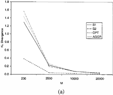
We considered the situation where the DM knows the pri­ ors used by the sources and adjusts for the unduly large number of imaginary samples. All sources and OMs used the Dirichlet prior defined by the uniform distribution and an estimated sample size of I. We varied the total num­ ber of samples M between 200 and 20000, having sources see the same number of samples in some cases and dif­ ferent numbers in others. We conducted multiple runs for each setting and averaged them. Figure 2(a) plots the av­ erages for the Alarm network when sources have equal ai. Due to software limitations, we had to start each structure search with the fully disconnected graph and used no ran­ dom restarts for this larger network. As can be seen, in spite of the limited search, our algorithm does fairly well as far as coming close to the optimal and improving on the sources. Not surprisingly, the KL divergence drops as the total number of samples increases. Furthermore, the exper­ iments on sources with different ai showed no dependence of the performance of the algorithm on the relative differ­ ence in ai.

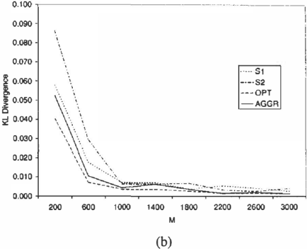
We ran similar experiments on Asia. Here, we varied the number of samples between 200 and 3000, with five runs per setting. For each run, we used five random restarts. Figure 2(b) plots the average for each setting. The plot shows that when we are able to explore the search space sufficiently in the learning and aggregation algorithms, our algorithm consistently improves on the sources and closely approximates to the optimal.

3 Available at http://www.cs.berkeley.edu/ murphyklbnt.htmL 4The KL divergence of distribution q from p is defined as LwewP(w)log �-

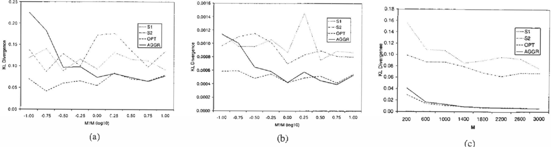
5.2 Sensitivity to the DM's estimation of M

We hypothesized earlier that the actual value of the OM's estimate of M does not matter all that much. To demon­ strate this, we ran experiments on the Asia network similar to those above, but leaving M fixed and varying the OM's estimate 1 order of magnitude above and below M. Fig­ ures 3(a) summarizes the results forM = 100.

Any approximation above 0.25 orders of magnitude below M provides improvement over the sources. Estimates be­ low this made the complexity penalty sufficiently strong to select DAGs with fewer arcs than the original and under­ fit the data. On the other hand, although overestimating M did not increase the KL distance from the original, there is a danger of extreme overestimates causing overfitting. How­ ever, we did not find any increase in the complexity of the aggregate networks for the I order of magnitude range we considered; they remained at 8-9 arcs on average.

0.20 ...----�

0.0016 r-----.

(c)

Figure 3: Asia network results (a) varying DM's estimate of M (M = 100). (b) varying DM's estimate of M (M = lOk). (c) with different subpopulations.

that, as predicted, the range of "slack" increases with M; the more samples seen by the sources, the less important the accuracy of the DM's estimate.

5.3 Subpopulations

Our algorithm performs well when combining source dis­ tributions learned based on samples from different subpop­ ulations. To show this, we modified the Asia network to ac­ comodate two sources, a doctor practicing in San Francisco and one practicing in Cincinnati. The probability distribu­ tions of the two root nodes in the Asia network, represent­ ing whether a patient smokes and whether she has visited Asia would be significantly different for the two doctors. A patient from San Francisco is less likely to be a smoker, and one from Cincinnati is less likely to have visited Asia. Thus, we added a source variable as described in Section 2, gave the sources equal priors of seeing patients, made the source variable a parent of the two root variables, and gave them appropriate CPDs. We drew M samples from this extended network and had each source learn from the ap­ propriate subset, then used AGGR to combine the results using the correct ai and M. Figure 3(c) plots the KL di­ vergence of each distribution from the original distribution with the source variable marginalized out. Because the sources are learning the distributions for different subpop­ ulations, what they learn is relatively far from the overall distribution. The DM takes advantage of the information from both sources and learns a BN that approximates the original much more closely than either source.

5.4 Comparison to sampling algorithm

In each of the above experiments, we also compared the performance of our algorithm to the alternative intuitive al­ gorithm SAMP we described in Section 4.2 in which we sample aiM samples from each source i's BN and learn a BN from the combined data. SAMP did very badly in general, consistently worse than not only AGGR, but worse than the sources as well, often by an order of magnitude.

6 Related Work

A wealth of work exists in statistics on aggregating prob­ ability distributions. Good surveys of the field include [GZ86, CW99]. Many of the earlier, axiomatic approaches suffered from a lack of semantical grounding. For this rea­ son, the community moved towards modeling approaches instead. The most studied approach has been the supra­ Bayesian one, introduced in [Win68] and formally estab­ lished in [Mor74, Mor77]. Here, the DM has a prior not only over the variables in the domain, but over the possi­ ble beliefs of the sources as well. She aggregates by us­ ing Bayesian conditioning to incorporate the information she receives from the sources. In fact, Proposition 1 de­ rives from this body of work. However, almost all of this work has been restricted to aggregating beliefs represented as point probabilities or odds, or joint distributions.

There has been some recent interest, particularly in AI, in the problem of aggregating structured distributions includ­ ing [MA92, MA93, PW99]. But, like the early axiomatic approaches in statistics, much of this work focuses on at­ tempting to satisfy abstract properties such as preserving shared independences, and often runs into impossibility re­ sults as a consequence.

In some sense, what we are doing could also be viewed as ensemble learning for BNs. Ensemble learning involves combining the results of different weak learners to improve classification accuracy. Because of its simplicity, LinOP is often used without justification to do the actual combina­ tion. Our results justify this use when the weak learners use MLE, MAP, or BN learning.

Another new area in AI that bears similarities to our work is that of on-line or incremental learning of BNs (e.g.,

[Bun91, LB94, FG97]). There, we are given a continuous stream of samples and we want to maintain a BN learned from all the data we have seen so far. Because the stream is very long, it is generally not possible to maintain the full set of sufficient statistics. Approaches range from approximat­ ing the sufficient statistics to restricting the network that can be learned. We essentially do the former by assuming that the sufficient statistics for the data seen by each source is encoded in its network. Cross-fertilization between the two fields may prove profitable.

7 Conclusion

We have presented a new approach to belief aggregation. We believe that we cannot formulate that problem pre­ cisely or measure success of different techniques without answering questions about the way in which sources' be­ liefs were formulated. We argued that a framework in which the sources are assumed to have learned their distri­ butions from data is both intuitively plausible and leads to a very natural formulation of the optimal DM distribution one which would be learned from the combined data sets -and a natural success measure - a distance from the generating, 'true ' distribution.

Based on the observation that LinOP is the appropriate operator for this framework if sources and DM are MLE learners, we presented a LinOP-based algorithm to aggre­ gate beliefs represented by Bayesian networks. Our prelim­ inary results show that this algorithm performs very well.

One direction of future work will involve finding ways to relax the various assumptions. For example, we would like to extend the framework to allow for continuous variables and to allow for dependence between sources' sample sets.

In our framework, the DM completely ignores sources' pri­ ors. This may be appropriate if the priors are known to be unreliable or uninformative. However, the priors used in real applications are often informative in and of themselves. Thus, a second direction will involve finding valid ways of taking advantage of sources' priors to improve the quality of the aggregation. For example, if sources use Dirichlet priors and the DM trusts their estimated sample sizes, she may chose to incorporate them into her estimate of M.

Acknowledgements

Pedrito Maynard-Reid II was partially supported by a Na­ tional Physical Science Consortium Fellowship. Urszula Chajewska was supported by the Air Force contract F30602-00-2-0598 under DARPA's TASK program.

References

[BS CC 89 ] I. Beinlich, G. Suerrnondt, R. Chavez, and G. Cooper. The ALARM monitoring system. In

Proc. European Conf. on AI and Medicine, 1989.

• [Bun91] W. Buntine. Theory refinement on bayesian net­ works. In Proc. UA/'91, pages 52-60, 1991.
• [CW99] R. T. Clemen and R. L. Winkler. Combining proba­ bility distributions from experts in risk analysis. Risk Analysis, 19(2):187-203, 1999.
• [FG97] N. Friedman and M. Goldsmidt. Sequential update of bayesian network structure. In Proc. UA/'97, pages

165-174, 1997.

• [FH96] N. Friedman and J. Y. Halpern. critique. In Proc. KR'96, pages 421-431, 1996.

Belief revision: A

• [GZ86] C. Genest and J. V. Zidek. Combining probability distributions: A critique and an annotated bibliography. Statistical Science, 1(1):114-148, 1986.

[Hec96] D. Heckerrnan. A tutorial on learning bayesian net­

works. Technical Report MSR-TR-95-06, Microsoft Research, 1996.

[HHN92] D. Heckerrnan, E. Horvitz, and B. Nathwani. Toward normative expert systems: Part I. The Pathfinder project. Methods of lnfonnation in Medicine, 31:90105, 1992.

• [Kul59] S. Kullback. lnfonnation Theory and Statistics. Wi­ ley, 1959.
• [LB94]

W. Lam and F. Bacchus. Learning bayesian belief networks: An approach based on the mdl principle. Computational Intelligence, 10:269-293, 1994.

[LS88] S. L. Lauritzen and D. J. Spiegelhalter. Local compu­ tations with probabilities on graphical structures and their application to expert systems. In 1. Royal Sta­ tistical Society, Series B (Methodological), volume 50(2), pages 157-224, 1988.

I. Matzkevich and B. Abramson. The topological fu­ sion of Bayes nets. In Proc. UA/'92, pages 191-198,

• [MA92] 1992.

[MA93]

I. Matzkevich and B. Abramson. Some complexity considerations in the combination of belief networks. In Proc. UA/'93, pages 152-158, 1993.

• [Mor74] P. A. Morris. Decision analysis expert use. Manage­ ment Science, 20:1233-1241, 1974.
• [Mor77] P. A. Morris. Combining expert judgements: A bayesian approach. Management Science, 23:679693, 1977.
• [Mor83] P. A. Morris. An axiomatic approach to expert reso­ lution. Management Science, 29(1):24-32, 1983.

Probabilistic Reasoning in Intelligent Sys­

• [Pea88] J. Pearl. tems. Morgan Kaufmann, 1988.

[PMGHOO] D. M. Pennock, P. Maynard-Reid IT, C. L. Giles, and E. Horvitz. A normative examination of ensemble learning algorithms. In Proc. ICML'OO, pages 735742,2000.

[PW99]

D. M. Pennock and M.P. Wellman. Graphical rep­ resentations of consensus belief. In Proc. UA/'99, pages 531-540, 1999.

[Sto61] M. Stone. The opinion pool. Annals of Mathematical Statistics, 32(4):1339-1342, 1961.

• [Win68] Robert L. Winkler. The consensus of subjec­ tive probability distributions. Management Science, 15(2):B61-B75, October 1968.