Contents
1207.0206
Alternative Restart Strategies for CMA-ES
Ilya Loshchilov 1 , 2 , Marc Schoenauer 1 , 2 , and Mich` ele Sebag 2 , 1
1 TAO Project-team, INRIA Saclay - ˆ /star/star
Ile-de-France 2 Laboratoire de Recherche en Informatique (UMR CNRS 8623) Universit´ e Paris-Sud, 91128 Orsay Cedex, France
Abstract. This paper focuses on the restart strategy of CMA-ES on multi-modal functions. A first alternative strategy proceeds by decreasing the initial step-size of the mutation while doubling the population size at each restart. A second strategy adaptively allocates the computational budget among the restart settings in the BIPOP scheme. Both restart strategies are validated on the BBOB benchmark; their generality is also demonstrated on an independent real-world problem suite related to spacecraft trajectory optimization.
1 Introduction
The long tradition of performance of the Covariance Matrix Adaptation Evolution Strategy (CMA-ES) algorithm on real-world problems (with over 100 published applications [6]) is due among others to its good behavior on multi-modal functions. Two versions of CMA-ES with restarts have been proposed to handle multi-modal functions: IPOP-CMA-ES [2] was ranked first on the continuous optimization benchmark at CEC 2005 [4,3]; and BIPOP-CMA-ES [5] showed the best results together with IPOP-CMA-ES on the black-box optimization benchmark (BBOB) in 2009 and 2010.
This paper focuses on analyzing and improving the restart strategy of CMAES, viewed as a noisy hyper-parameter optimization problem in a 2D space (population size, initial step-size). Two restart strategies are defined. The first one, NIPOP-aCMA-ES ( New IPOP-aCMA-ES), differs from IPOP-CMA-ES as it simultaneously increases the population size and decreases the step size. The second one, NBIPOP-aCMA-ES, allocates computational power to different restart settings depending on their current results. While these strategies have been designed with the BBOB benchmarks in mind [8], their generality is shown on a suite of real-world problems [16].
The paper is organized as follows. After describing the weighted active ( µ/µ w , λ )-CMA-ES and its current restart strategies (section 2), the proposed restart schemes are described in section 3. Section 4 reports on their experimental validation. The paper concludes with a discussion and some perspectives for further research.
/star/star Work partially funded by FUI of System@tic Paris-Region ICT cluster through contract DGT 117 407 Complex Systems Design Lab (CSDL).
2 The Weighted Active ( µ/µ w , λ )-CMA-ES
The CMA-ES algorithm is a stochastic optimizer, searching the continuous space R D by sampling λ candidate solutions from a multivariate normal distribution [10, 9]. It exploits the best µ solutions out of the λ ones to adaptively estimate the local covariance matrix of the objective function, in order to increase the probability of successful samples in the next iteration. The information about the remaining (worst λ -µ ) solutions is used only implicitly during the selection process.
In active ( µ/µ I , λ )-CMA-ES however, it has been shown that the worst solutions can be exploited to reduce the variance of the mutation distribution in unpromising directions [12], yielding a performance gain of a factor 2 for the active ( µ/µ I , λ )-CMA-ES with no loss of performance on any of tested functions. A recent extension of the ( µ/µ w , λ )-CMA-ES, weighted active CMA-ES [11] (referred to as aCMA-ES for brevity) shows comparable improvements on a set of noiseless and noisy functions from the BBOB benchmark suite [7]. In counterpart, aCMA-ES no longer guarantees the covariance matrix to be positive definite, possibly resulting in algorithmic instability. The instability issues can however be numerically controlled during the search; as a matter of fact they are never observed on the BBOB benchmark suite.
At iteration t , ( µ/µ w , λ )-CMA-ES samples λ individuals according to
where N ( m , C ) denotes a normally distributed random vector with mean m and covariance matrix C .
These λ individuals are evaluated and ranked, where index i : λ denotes the i -th best individual after the objective function. The mean of the distribution is updated and set to the weighted sum of the best µ individuals ( m = ∑ µ i =1 w i x ( t ) i : λ , with w i > 0 for i = 1 . . . µ and µ i =1 w i = 1).
where y λ -i : λ = ∥ ∥ ∥ C t -1 / 2 ( x λ -µ +1+ i : λ -m t ) ∥ ∥ ∥ ‖ C t -1 / 2 ( x λ -i : λ -m t ) ‖ × x λ -i : λ -m t σ t . The covariance matrix estimation of these worst solutions is used to decrease the variance of the mutation
∑ The active CMA-ES only differs from the original CMA-ES in the adaptation of the covariance matrix C ( t ) . Like for CMA-ES, the covariance matrix is computed from the best µ solutions, C + µ = ∑ µ i =1 w i x i : λ -m t σ t × ( x i : λ -m t ) T σ t . The main novelty is to exploit the worst solutions to compute C -µ = ∑ µ -1 i =0 w i +1 y λ -i : λ y T λ -i : λ , distribution along these directions:
where p t +1 c is adapted along the evolution path and coefficients c 1 , c µ , c -and α -old are defined such that c 1 + c µ -c -α -old ≤ 1. The interested reader is referred to [10, 11] for a more detailed description of these algorithms.
As mentioned, CMA-ES has been extended with restart strategies to accommodate multi-modal fitness landscapes, and to specifically handle objective functions with many local optima. As observed by [9], the probability of reaching the optimum (and the overall number of function evaluations needed to do so) is very sensitive to the population size. The default population size λ default has been tuned for uni-modal functions; it is hardly large enough for multi-modal functions. Accordingly, [2] proposed a 'doubling trick' restart strategy to enforce global search: the restart ( µ/µ w , λ )-CMA-ES with increasing population, called IPOP-CMA-ES, is a multi-restart strategy where the population size of the run is doubled in each restart until meeting a stopping criterion.
The BIPOP-CMA-ES instead considers two restart regimes. The first one, which corresponds to IPOP-CMA-ES, doubles the population size λ large = 2 i restart λ default in each restart i restart and uses a fixed initial step-size σ 0 large = σ 0 default .
The second regime uses a small population size λ small and initial step-size σ 0 small , which are randomly drawn in each restart as:
where U [0 , 1] stands for the uniform distribution in [0 , 1]. Population size λ small thus varies ∈ [ λ default , λ large / 2]. BIPOP-CMA-ES launches the first run with default population size and initial step-size. In each restart, it selects the restart regime with less function evaluations. Clearly, the second regime consumes less function evaluations than the doubling regime; it is therefore launched more often.
3 Alternative Restart Strategies
3.1 Preliminary Analysis
The restart strategies of IPOP- and BIPOP-CMA-ES are viewed as a search in the hyper-parameter space.
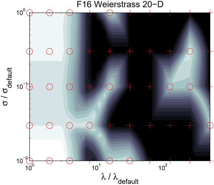
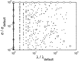
IPOP-CMA-ES only aims at adjusting population size λ . It is motivated by the results observed on multi-modal problems [9], suggesting that the population size must be sufficiently large to handle problems with global structure. In such cases, a large population size is needed to uncover this global structure and to lead the algorithm to discover the global optimum. IPOP-CMA-ES thus increases the population size in each restart, irrespective of the results observed so far; at each restart, it launches a new CMA-ES with population size λ = ρ i restart inc λ default (see ◦ on Fig. 1). Factor ρ inc must be not too large to avoid 'overjumping' some possibly optimal population size λ ∗ ; it must also be not too small in order to reach λ ∗ in a reasonable number of restarts. The use of the doubling trick ( ρ inc = 2) guarantees that the loss in terms of function evaluations (compared to the 'oracle' restart strategy which would directly set the population size to the optimal value λ ∗ ) is about a factor of 2.
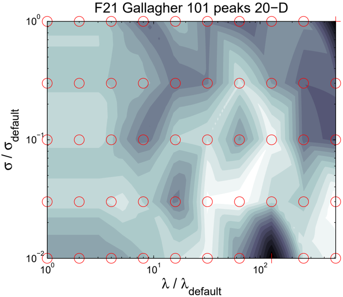
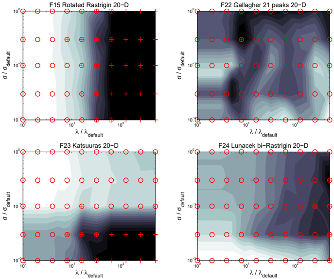
On the Rastrigin 20-D function, IPOP-CMA-ES performs well and always finds the optimum after about 5 restarts (Fig. 1, top-left). The Rastrigin function displays indeed a global structure where the optimum is the minimizer of this structure. For such functions, IPOP-CMA-ES certainly is the method of choice. For some other functions such as the Gallagher function, there is no such global structure; increasing the population size does not improve the results. On Katsuuras and Lunacek bi-Rastrigin functions, the optimum can only be found with small initial step-size (lesser than the default one); this explains why it can be solved by BIPOP-CMA-ES, sampling the two-dimensional ( λ, σ ) space.
Actually, the optimization of a multi-modal function by CMA-ES with restarts can be viewed as the optimization of the function h ( θ ), which returns the optimum found by CMA-ES defined by the hyper-parameters θ =( λ, σ ). Function
h ( θ ), graphically depicted in Fig. 1 can be viewed as a black box, computationally expensive and stochastic function (reflecting the stochasticity of CMA-ES). Both IPOP-CMA-ES and BIPOP-CMA-ES are based on implicit assumptions about the h ( θ ): IPOP-CMA-ES achieves a deterministic uni-dimensional trajectory, and BIPOP-CMA-ES randomly samples the 2-dimensional search space.
Function h ( θ ) also can be viewed as a multi-objective fitness, since in addition to the solution found by CMA-ES, h ( θ ) could return the number of function evaluations needed to find that solution. h ( θ ) could also return the computational effort SP1 (i.e. the average number of function evaluations of all successful runs, divided by proportion of successful runs). However, SP1 can only be known for benchmark problems where the optimum is known; as the empirical optimum is used in lieu of true optimum, SP1 can only be computed a posteriori .
3.2 Algorithm
Two new restart strategies for CMA-ES, respectively referred to as NIPOPaCMA-ES and NBIPOP-aCMA-ES, are presented in this paper.
If the restart strategy is restricted to the case of increasing of population size (IPOP), we propose to use NIPOP-aCMA-ES, where we additionally decrease the initial step-size by some factor ρ σdec . The rationale behind this approach is that the CMA-ES with relatively small initial step-size is able to explore small basins of attraction (see Katsuuras and Lunacek bi-Rastrigin functions on Fig. 1), while with initially large step-size and population size it will neglect the local structure of the function, but converge to the minimizer of the global structure. Moreover, initially, relatively small step-size will quickly increase if it makes sense, and this will allow the algorithm to recover the same global search properties than with initially large step-size (see Rastrigin function on Fig. 1).
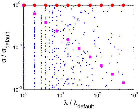
NIPOP-CMA-ES thus explores the two-dimensional hyper-parameter space in a deterministic way (see /square symbols on Fig. 2). For ρ σdec = 1 . 6 used in this study, NIPOP-CMA-ES thus reaches the lower bound ( σ = 10 -2 σ default ) used by BIPOP-CMA-ES after 9 restarts, expectedly reaching the same performance as BIPOP-CMA-ES albeit it uses only a large population.
The second restart strategy, NBIPOP-aCMA-ES, addresses the case where the probability to find the global optimum does not much vary in the ( λ, σ ) space. Under this assumption, it makes sense to have many restarts for a fixed budget (number of function evaluations). Specifically, NBIPOP-aCMA-ES implements the competition of the NIPOP-aCMA-ES strategy (increasing λ and decreasing initial σ 0 in each restart) and a uniform sampling of the σ space, where λ is set to λ default and σ 0 = σ 0 default × 10 -2 U [0 , 1] The selection between the two (NIPOPaCMA-ES and the uniform sampling) depends on the allowed budget like in NBIPOP-aCMA-ES. The difference is that NBIPOP-aCMA-ES adaptively sets the budget allowed to each restart strategy, where the restart strategy leading to the overall best solution found so far is allowed twice ( ρ budget = 2) a budget compared to the other strategy.
4 Experimental Validation
The experimental validation of NIPOP-aCMA-ES and NBIPOP-aCMA-ES investigates the performance of the approach comparatively to IPOP-aCMA-ES and BIPOP-aCMA-ES on BBOB noiseless problems and one black-box realworld problem related to spacecraft trajectory optimization. The default parameters of CMA-ES [11, 5] are used. This section also presents the first experimental study of BIPOP-aCMA-ES 3 , the active version of BIPOP-CMA-ES [5].
4.1 Benchmarking with BBOB Framework
The BBOB framework [7] is made of 24 noiseless and 30 noisy functions [8]. Only the noiseless case has been considered here. Furthermore, only the 12 multimodal functions among these 24 noiseless functions are of interest for this study, as CMA-ES can solve the 12 other functions without any restart.
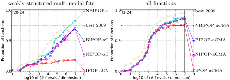
With same experimental methodology as in [7], the results obtained on these benchmark functions are presented in Fig. 4 and Table 1. The results are given for dimension 40, because the differences are larger in higher dimensions. The expected running time (ERT) , used in the figures and table, depends on a given target function value, f t = f opt + ∆f . It is computed over all relevant trials as the number of function evaluations required in order to reach f t , summed over all 15 trials, and divided by the number of trials that actually reached f t [7].
NIPOP-aCMA-ES . On 6 out of 12 test functions ( f 15 , f 16 , f 17 , f 18 , f 23 , f 24 ) NIPOP-aCMA-ES obtains the best known results for BBOB-2009 and BBOB2010 workshops. On f 23 Katsuuras and f 24 Lunacek bi-Rastrigin, NIPOP-aCMAES has a speedup of a factor from 2 to 3, as could have been expected. It performs
3 For the sake of reproducibility, the source code for NIPOP-aCMA-ES and NBIPOPaCMA-ES is available at https://sites.google.com/site/ppsnbipop/
unexpectedly well on f 16 Weierstrass functions, 7 times faster than IPOP-aCMAES and almost 3 times faster than BIPOP-aCMA-ES. Overall, according to Fig. 4, NIPOP-aCMA-ES performs as well as BIPOP-aCMA-ES, while restricted to only one regime of increasing population size.
NBIPOP-aCMA-ES . Thanks to the first regime of increasing population size, NBIPOP-aCMA-ES inherits some results of NIPOP-aCMA-ES. However, on functions where the population size does not play any important role, it performs significantly better than BIPOP-aCMA-ES. This is the case for f 21 Gallagher 101 peaks and f 22 Gallagher 21 peaks functions, where NBIPOPaCMA-ES has a speedup of a factor of 6. It seems that the adaptive choice between two regimes works efficiently on all functions except on f 16 Weierstrass. In this last case, NBIPOP-aCMA-ES mistakingly prefers small populations, with a loss factor 4 compared to NIPOP-aCMA-ES. According to Fig. 4, NBIPOPaCMA-ES performs better than BIPOP-aCMA-ES on weakly structured multimodal functions, showing overall best results for BBOB-2009 and BBOB-2010 workshops in dimensions 20 (results not shown here) and 40.
Due to space limitations, the interested reader is referred to [13] for a detailed presentation of the results.
4.2 Interplanetary Trajectory Optimization
The NIPOP-aCMA-ES and NBIPOP-aCMA-ES strategies, designed for the BBOB benchmark functions, can possibly overfit this benchmark suite. In order to test the generality of these strategies, a real-world black-box problem is considered, pertaining to a completely different domain: Advanced Concepts Team of European Space Agency is making available several difficult spacecraft trajectory optimization problems as black box functions to invite the operational research community to compare different derivative-free solvers on these test problems [16].
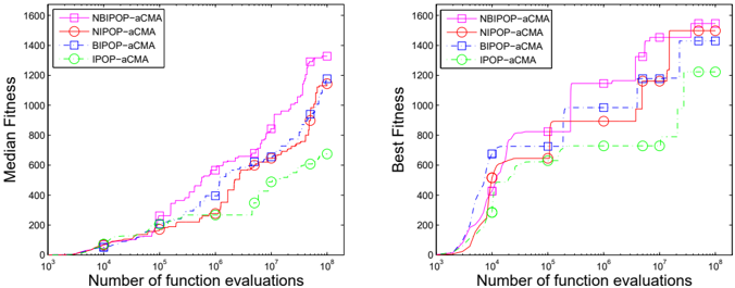
The following results consider the 18-dimensional bound-constrained blackbox function 'TandEM-Atlas501', that defines an interplanetary trajectory to Saturn from the Earth with multiple fly-bys, launched by the rocket Atlas 501. The final goal is to maximize the mass f ( x ), which can be delivered to Saturn using one of 24 possible fly-by sequences with possible maneuvers around Venus, Mars and Jupiter.
The first best results was found for a sequence Earth-Venus-Earth-EarthSaturn ( f max = 1533 . 45) in 2008 by B. Addis et al. [1]. The best results so far ( f max = 1673 . 88) was found in 2011 by G. Stracquadanio et al. [15].
All versions of CMA-ES with restarts have been launched with a maximum budget of 10 8 function evaluations. All variables are normalized in the range [0 , 1]. In the case of sampling outside of boundaries, the fitness is penalized and becomes f ( x ) = f ( x feasible ) -α ‖ x -x feasible ‖ 2 , where x feasible is the closest feasible point from point x and α is a penalty factor, which was arbitrarily set to 1000.
As shown on Fig. 3, the new restart strategies NIPOP-aCMA-ES and NBIPOPaCMA-ES respectively improve on the former ones (IPOP-aCMA-ES and BIPOP-
aCMA-ES); further, NIPOP-aCMA-ES reaches same performances as BIPOPaCMA-ES.
The best solution found by NBIPOP-aCMA-ES 4 improves on the best solution found in 2008, while it is worse than the current best solution, which is blamed on the lack of problem specific heuristics [1, 15], on the possibly insufficient time budget (10 8 fitness evaluations), and also on the lack of appropriate constraint handling heuristics.
5 Conclusion and Perspectives
This paper contribution regards two new restart strategies for CMA-ES. NIPOPaCMA-ES is a deterministic strategy simultaneously increasing the population size and decreasing the initial step-size of the Gaussian mutation. NBIPOPaCMA-ES implements a competition between NIPOP-aCMA-ES and a random sampling of the initial mutation step-size, adaptively adjusting the computational budget of each one depending on their current best results. Besides the extensive validation of NIPOP-aCMA-ES and NBIPOP-aCMA-ES on the BBOB benchmark, the generality of these strategies has been tested on a new problem, related to interplanetary spacecraft trajectory planning.
The main limitation of the proposed restart strategies is to quasi implement a deterministic trajectory in the θ space. Further work will consider h ( θ ) as yet another expensive noisy black-box function, and the use of a CMA-ES in the hyper-parameter space will be studied. The critical issue is naturally to keep
4 x =[0.83521, 0.45092, 0.50284, 0.65291, 0.61389, 0.75773, 0.43376, 1, 0.89512, 0.77264, 0.11229, 0.20774, 0.018255, 6.2057e-09, 4.0371e-08, 0.2028, 0.36272, 0.32442]; fitness(x) = mass(x) = 1546.5
the overall number of fitness evaluations beyond reasonable limits. A surrogatebased approach will be investigated [14], learning and exploiting an estimate of the (noisy and stochastic) h ( θ ) function.
References
- B. Addis, A. Cassioli, M. Locatelli, , and F. Schoen. Global optimization for the design of space trajectories. Optimization On Line , 11, 2008.
- A. Auger and N. Hansen. A restart CMA evolution strategy with increasing population size. In Proceedings of the IEEE Congress on Evolutionary Computation (CEC 2005) , pages 1769-1776. IEEE Press, 2005.
- S. Garc´ ıa, D. Molina, M. Lozano, and F. Herrera. A study on the use of nonparametric tests for analyzing the evolutionary algorithms' behaviour: a case study on the CEC'2005 special session on real parameter optimization. Journal of Heuristics , 15:617-644, 2009.
- N. Hansen. Compilation of results on the 2005 CEC benchmark function set. Online, May 2006.
- N. Hansen. Benchmarking a BI-population CMA-ES on the BBOB-2009 function testbed. In F. Rothlauf, editor, GECCO Companion , pages 2389-2396. ACM, 2009.
- N. Hansen. References to CMA-ES applications. http://www.lri.fr/ hansen/cmaapplications.pdf, 2009.
- N. Hansen, A. Auger, S. Finck, and R. Ros. Real-parameter black-box optimization benchmarking 2012: Experimental setup. Technical report, INRIA, 2012.
- N. Hansen, S. Finck, R. Ros, and A. Auger. Real-parameter black-box optimization benchmarking 2009: Noiseless functions definitions. Technical Report RR-6829, INRIA, 2009. Updated February 2010.
- N. Hansen and S. Kern. Evaluating the cma evolution strategy on multimodal test functions. In PPSN'04 , pages 282-291, 2004.
- N. Hansen and A. Ostermeier. Completely derandomized self-adaptation in evolution strategies. Evolutionary Computation , 9(2):159-195, 2001.
- N. Hansen and R. Ros. Benchmarking a weighted negative covariance matrix update on the BBOB-2010 noiseless testbed. In GECCO '10: Proceedings of the 12th annual conference comp on Genetic and evolutionary computation , pages 16731680, New York, NY, USA, 2010. ACM.
- G. A. Jastrebski and D. V. Arnold. Improving evolution strategies through active covariance matrix adaptation. In IEEE Congress on Evolutionary Computation CEC 2006 , pages 2814-2821, 2006.
- I. Loshchilov, M. Schoenauer, and M. Sebag. Black-box Optimization Benchmarking of NIPOP-aCMA-ES and NBIPOP-aCMA-ES on the BBOB-2012 Noiseless Testbed. In GECCO '2012: Proceedings of the 14th annual conference on Genetic and evolutionary computation , page to appear. ACM, 2012.
- I. Loshchilov, M. Schoenauer, and M. Sebag. Self-Adaptive Surrogate-Assisted Covariance Matrix Adaptation Evolution Strategy. In GECCO '2012 Proceedings , page to appear. ACM, 2012.
- G. Stracquadanio, A. La Ferla, M. De Felice, and G. Nicosia. Design of robust space trajectories. In Research and Development in Intelligent Systems XXVIII , pages 341-354. Springer Verlag, 2011.
- T. Vinko and D. Izzo. Global Optimisation Heuristics and Test Problems for Preliminary Spacecraft Trajectory Design. Technical Report GOHTPPSTD, European Space Agency, 2008.
| ∆f opt | 1e1 | 1e0 | 1e-1 | 1e-3 | 1e-5 | 1e-7 | #succ | ∆f opt | 1e1 | 1e0 | 1e-1 | 1e-3 | 1e-5 | 1e-7 | #succ |
|---|---|---|---|---|---|---|---|---|---|---|---|---|---|---|---|
| f3 | 15526 | 15602 ∞ | 15612 ∞ | 15646 ∞ | 15651 | ∞ 4e7 | 1565615/15 0/15 | f19 BIPOP-a 396 | 1 | 1 | 1.4e6 | 2.6e7 | 4.5e7 | 4.5e7 1.0 | 8/15 |
| BIPOP-a 2395 IPOP-aC | 8177 | ∞ ∞ | ∞ | ∞ ∞ | ∞ ∞ ∞ | ∞ 6e6 ∞ 4e7 | 0/8 0/15 | IPOP-aC NBIPOP- | 462 | 6.7e4 8.3e4 | 0.87 4.4e40.57 | 1.2 0.34 | 1.0 0.20 1.1 | 0.20 1.1 | 9/15 8/8 9/15 |
| ∞ NBIPOP- NIPOP-a | 4615 | ∞ | ∞ ∞ | 424 | 0.97 | 0.81 | 15/15 | ||||||||
| ∆f | ∞ | ∞ | ∞ 4e7 | 0/15 | NIPOP-a | 436 | 8.2e4 1.9 | 0.48 | 0.32 | 0.32 | |||||
| opt | 1e1 | 1e0 | 1e-1 | 1e-3 | 1e-5 | 1e-7 | #succ | ∆f opt | 1e1 | 1e0 | 1e-1 | 1e-3 | 1e-5 | 1e-7 | #succ |
| f4 BIPOP-a | 15536 | 15601 | 15659 | 15703 ∞ | 15733 ∞ | 2.8e5 ∞ | 6/15 | f20 BIPOP-a | 222 | 1.3e5 | 1.6e8 | ∞ | ∞ | ∞ | 0 0/15 |
| IPOP-aC | ∞ | ∞ ∞ | ∞ ∞ | ∞ | 4e7 ∞ 6e6 | 0/15 0/8 | 4.0 | 9.0 | 0.34 | . | . | . | |||
| NBIPOP- | ∞ | ∞ ∞ | ∞ | IPOP-aC | 3.9 | 8.1 | 0.18 | . | . | . | 0/8 | ||||
| ∞ | ∞ | ∞ | ∞ | 4e7 | 0/15 | NBIPOP-4.0 | 8.5 | 0.39 | . | . | . | 0/15 | |||
| NIPOP-a | ∞ | ∞ | ∞ | ∞ | ∞ | ∞ 4e7 | 0/15 | NIPOP-a | 4.0 | 6.5 | 0.32 | . | . | . | 0/15 |
| ∆f opt | 1e1 | 1e0 | 1e-1 | 1e-3 | 1e-5 | 1e-7 | #succ | ∆f opt | 1e1 | 1e0 | 1e- | 1e- | 1e- 5 | 1e- 7 | #succ |
| f15 BIPOP-a | 1.9e5 1.2 0.72 | 7.9e5 1.1 | 1.0e6 1.1 | 1.1e6 1.1 | 1.1e6 1.1 | 1.1e6 1.1 | 15/15 15/15 | f21 BIPOP-a | 1044 | 21144 | 1 1.0e5 | 3 1.0e5 | 1.0e5 | 1.0e5 | 26/30 15/15 |
| IPOP-aC | 0.92 | 0.43 0.71 0.61 | 0.60 0.75 | 0.61 0.76 0.56 | 0.62 0.77 0.57 | 0.63 0.77 0.58 | 8/8 15/15 15/15 | IPOP-aC NBIPOP- | 7.5 7.1 4.9 | 60 10 | 37 ∞ 5.1 | 37 ∞ 5.1 | 37 ∞ 5.1 | 37 ∞ 5.1 | 0/8 15/15 |
| NBIPOP-1.0 NIPOP-a | 421 | 3e6 | |||||||||||||
| ∆f opt f16 | 1e1 | 1e0 | 0.55 | 1e-3 | 1e-5 | 1e-7 | #succ | NIPOP-a ∆f | 14 | 440 | 173 | 171 | 171 | 12/15 | |
| 1e-1 | opt | 1e1 | 1e- | 172 | 1e- | 1e- | #succ | ||||||||
| BIPOP-a | 5244 1.3 | 72122 0.96 | 3.2e5 0.80 | 1.4e6 0.54 | 2.0e6 0.50 | 2.0e6 0.51 | 15/15 15/15 | f22 | 1e0 | 1 | 1e- 3 | 5 | 7 6.5e5 | 8/30 4/15 | |
| IPOP-aC NBIPOP-0.97 | 0.91 | 1.1 | 1.0 | 0.51 0.38 | 1.4 0.46 | 1.4 0.74 | 8/8 15/15 | BIPOP-a | 3090 12 | 35442 | 6.5e5 201 | 6.5e5 200 | 6.5e5 200 | 199 | |
| NIPOP-a | 1.2 1e1 | 0.78 0.65 | 0.34 0.23 | 0.21 | 0.16 | 0.18 | 15/15 | IPOP-aC | 144 | 343 93 | ∞ | ∞ 32 | ∞ 32 | ∞ 3e6 32 | 0/8 |
| ∆f opt f17 | 399 | 1e0 | 1e-1 | 1e-3 | 1e-5 | 1e-7 | #succ 14/15 | NBIPOP- NIPOP-a | 12 179 | 112 583 | 32 ∞ | ∞ | ∞ | ∞ 4e7 | 12/15 0/15 |
| BIPOP-a | 1.1 | 4220 0.64 | 14158 1.6 | 51958 1.1 | 1.3e5 | 2.7e5 | 15/15 | ∆f opt | 1e1 | 1e0 | 1e-3 | 1e-7 | #succ | ||
| IPOP-aC | 1.0 | 0.52 | 1.3 | 1.4 | 0.87 | 8/8 | f23 | 7.1 | 11925 | 1e-1 75453 | 1.3e6 | 1e-5 3.2e6 | 3.4e6 | 15/15 | |
| NIPOP-a | 0.57 | 1.2 | 1.3 1.2 | 0.97 1.0 | 0.83 0.81 | 15/15 | BIPOP-a | 7.8 | 1.3 | 1.9 | 1.00 | 0.99 ∞ | 15/15 | ||
| NBIPOP-1.0 | 0.97 | 0.52 | 0.97 | 1.00 | 1.1 | 0.70 | 15/15 | IPOP-aC | 8.4 9.2 | ∞ | ∞ | ∞ | ∞ | 4e6 | 0/8 |
| ∆f opt f18 | 1e1 | 1e0 | 1e-1 | 1e-3 | 1e-5 | 1e-7 | #succ | NBIPOP-8.6 | 10 | 1.6 | 1.3 | 0.58 0.36 | 0.59 | 15/15 | |
| BIPOP-a | 1442 0.94 | 16998 | 47068 | 1.9e5 | 6.7e5 | 9.5e5 | 15/15 | NIPOP-a | 5.9 | 61 | 11 | 0.72 | 0.38 | 15/15 | |
| 0.51 | 1.0 | 0.98 | 15/15 | ∆f opt | 1e1 | 1e0 | 1e-1 | 1e-3 | 1e-5 | 1e-7 | #succ | ||||
| IPOP-aC | 0.96 | 0.68 | 1.0 | 0.66 | 0.88 | 0.67 | 8/8 | f24 | 3.0e8 | 3.0e8 | 3.0e8 | 3.0e8 | 1/15 | ||
| NBIPOP-1.0 | 0.97 | 1.1 | 0.93 | 0.45 | 0.48 0.53 | 15/15 | 5.8e6 | 9.8e7 | ∞ | ∞ | ∞ | ∞ 4e7 | 0/15 | ||
| 0.57 | BIPOP-a | 3.6 | 1.4 | ||||||||||||
| NIPOP-a | 0.95 | 0.58 | 15/15 | IPOP-aC | ∞ | ∞ | ∞ | ∞ | ∞ | ∞ 1e7 | 0/8 | ||||
| 0.97 | 0.97 | 2/15 | |||||||||||||
| 0.19 | 0.97 | 0.97 | 4/15 | ||||||||||||
| 0.75 | 0.71 | 0.50 | 0.42 | 1.2 | 0.15 | 0.44 | 0.44 | 0.44 | 0.44 | ||||||
| NBIPOP-2.1 | |||||||||||||||
| NIPOP-a | |||||||||||||||