An Anytime Algorithm for Decision Making under Uncertainty

Michael C. Horsch [email protected]

David Poole [email protected]

Department of Computer Science University of British Columbia 2366 Main Mall,

Vancouver, B.C., Canada V6T 1Z4

Abstract

We present an anytime algorithm which com­ putes policies for decision problems represented as multi-stage influence diagrams. Our algo­ rithm constructs policies incrementally, starting from a policy which makes no use of the avail­ able information. The incremental process con­ structs policies which includes more of the infor­ mation available to the decision maker at each step. While the process converges to the opti­ mal policy, our approach is designed for situa­ tions in which computing the optimal policy is in­ feasible. We provide examples of the process on several large decision problems, showing that, for these examples, the process constructs valuable (but sub-optimal) policies before the optimal pol­ icy would be available by traditional methods.

1 INTRODUCTION

The representational tools which decision analysts and AI practitioners have devised can represent large deci­ sion problems. When costs of computation are not taken into account, optimal policies can be determined using dy­ namic programming [Howard & Matheson, 1984; Shachter, 1986]. When the costs of computation are not negligible, the cost of computing the optimal policy using dynamic programming may be prohibitive.

We have developed an algorithm which can be used to com­ pute policies for large multi-stage decision problems un­ der uncertainty represented as influence diagrams. Our ap­ proach is incremental, and uses abstraction. The algorithm is sufficiently general to make use of existing tools for prob­ abilistic reasoning, and has already provided reasonably valuable (but non-optimal) policies for influence diagrams with about 261 states.

The algorithm is an extension of the iterative refinement technique presented in [Horsch & Poole, 1996], applied to multi-stage influence diagrams. The refinement is applied to the decision nodes in random access ordering (as op­ posed to the sequential ordering of dynamic programming).

This paper is organized as follows. First we briefly discuss influence diagrams and the decision tree representation of decision functions. Section 2 presents the random access algorithm. Empirical results are presented in Section 3.

1.1 INFLUENCE DIAGRAMS

An influence diagram (ID) is a DAG representing a sequen­ tial decision problem under uncertainty [Howard & Math­ eson, 1984]. An ID models the subjective beliefs, prefer­ ences, and available actions from the perspective of a single decision maker.

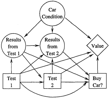
Nodes in an ID are of three types. Random variables, which the decision maker cannot control, are represented by circle shaped chance nodes. Decisions, i.e., sets of mutually ex­ clusive actions which the decision maker can take, are rep­ resented by square shaped decision nodes. The set of out­ comes (or actions) which can be taken by a chance node X (or decision node D ) is specified by Ox (or Ov).

The diamond shaped value node represents the decision maker's preferences in the form of a value function.

Arcs represent dependencies. A chance node is condition­ ally independent of its non-descendants given its direct pre­ decessors. The direct predecessors of a decision node will be called information predecessors; a value for each of these predecessors will be observed before an action must be taken. The decision maker's preferences are expressed as a function of the value node's direct predecessors. The set of a node's direct predecessor1? is specified by II sub­ scripted by the node's label.

Dependencies are accompanied by numerical information. There is a conditional probability table associated with ev­ ery chance node in the form P(XIUx) (unconditional, if it has no predecessors). The value node V has an associated value function, V : Orrv --+ lR, which may be represented as a table.

A policy prescribes an action (or sequence of actions, if there are several decision nodes) for each possible combi­ nation of outcomes of its information predecessors. The set !lrrn is the set of all possible combinations of values for de­ cision node D's information predecessors. An element in this set will be called an information state. A decision func­ tion for decision node Dis a mapping 8 : !lrrD ---+ nD. A policy for an ID is a set D. = { 8i, i = 1 . . . n} of decision functions, one for each decision node. ·

An optimal policy maximizes the decision maker's ex­ pected value, without regard to the cost of finding such a policy. If computational costs are not negligible, the deci­ sion maker's expected value might be maximized by a pol­ icy which is not optimal in this sense.

For example, the ID in Figure 1 represents the problem of deciding whether or not to buy a particular car. The decision maker has the option of performing a number of tests to var­ ious components of the car. The results of these tests will provide information to the decision to buy the car. The ac­ tual condition of the car is not observable directly at the time the decision maker must act, but influences the final value of the transaction. A policy for this problem would indicate which tests to do under which circumstances, as well as a prescription to buy the car (or not) given the results of the tests. Due to space constraints, none of the numerical data required to complete the specification of this problem is shown; this information can be found in [Qi & Poole, 1995; Smith, Holtzman, & Matheson, 1993].

In this paper, IDs are assumed to have chance and decision nodes with a finite number of discrete values. Furthermore, we limit the discussion to IDs with a single value node.

1.2 DECISION TREES

Let D be a decision node in an ID. A decision tree T for D is either a leaf labelled by an action dj E nD or a non­ leaf node labelled with some X E liD. Each non-leaf has a child decision tree for every value Xk E nx. An infor­ mation predecessor X E liD appears at most once in any path from the root to a leaf. Each vertex X in a decision tree has a context, 'YX, defined to be the conjunction of variable assignments on the path from the root of the tree to X. The action at the leaf represents the action to be taken in the con­ text of the leaf. Given an information state w E !lrrn, there is a corresponding path through a decision tree ford, start­ ing at the root leading to a leaf, which is labelled with the prescribed action to be taken in when w is observed.

Note that the context of an action need not contain an as­ signment for every variable in liD. In this case, the in­ formation has not been used in the decision function, even though it is available to the decision maker. In such a situ­ ation, a context is said to cover a set of information states.

A decision tree represents a decision function. We will refer to the action prescribed by a decision function by 8 ( w) for information state w, or by dz if lis a leaf on a given decision tree.

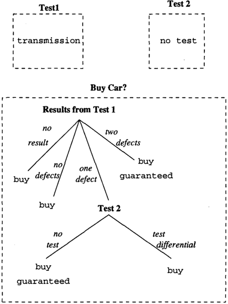
Figure 2 shows three decision trees, one tree for each de­ cision node in the Car Buyer problem (Figure 1). The de­ cision tree for Test 1 is a single leaf, which tells the decision maker to perform the test on the transmission. Since there are no information predecessors for this deci­ sion node, this decision tree is complete.

The decision tree for Test 2 tells the decision maker not to perform the test. Note that this decision node has 2 in­ formation predecessors. The decision tree does not make use of the available information; every information state is mapped to the action no test.

The decision tree for Buy Car? is a non-trivial tree, using two of four information predecessors. This decision func­ tion tells the decision maker to check the result from the first test: if there is no result or if there are no defects, the deci­ sion maker is directed to buy the car. If the result of Test 1 indicates one defect, the decision function uses the infor­ mation from the previous decision Test 2. If the decision to take the second test had been made, the decision maker should buy the car; if the decision maker did not have the second test performed, the car should be bought with a guar­ antee.

Note that not all of the information is used. A policy which used all of the available information naively would have 96 leaf vertices for Buy Car?; many of these would be log­ ically impossible due to the asymmetries of the problem. The problem is well known for its asymmetry, and the op­ timal policy can be represented by decision trees very suc­ cinctly.

1.3 THE SINGLE STAGE ALGORITHM

The single stage information refinement algorithm con­ structs a decision tree for a influence diagram with a sin­ gle decision node. The following description is a brief syn­ opsis. The algorithm has been described in more detail in [Horsch & Poole, 1996], and is similar to algorithms de­ scribed in [Heckerman, Breese, & Horvitz, 1989; Lehner & Sadigh, 1993].

For a given leaf l in a decision tree, its context 'Yl is exten­ sible if it does not contain all the information variables. We refer to the information variables which are not in the con­ text as possible extensions, writing 6. A decision tree t can be extended if there is a leaf with an extensible context; oth­ erwise, the tree is called complete.

The single stage algorithm can be summarized as follows: A decision tree is extended by removing an extensible leaf l having context 'Yl· This leaf is replaced with new a vertex X E 6. The new vertex X is given a new leaf for every value Xj E nx. Each leaf has a context /j which is the assignment of values (X = xi) A. 'Yl· Each leaf out of X will be labelled with an action di E nD. The action di is the action which maximizes the expected utility in the new context 'Yi = (X = xi) A. /l (this action will be called the MEV action for the leaf). The initial tree has one leaf, which is the MEV action to be taken in the empty context.

Other refinement operators are possible. For example, an extension might generate a branch for a particular value of X, and summarize the remaining values in a single branch. Determining how and when to use this kind of operator is an avenue for future research.

The sequence of trees created by the procedure is monoton­ ically non-decreasing in expected value. However, the pro­ cedure is myopic; there is no guarantee that the expected value will increase with every extension of the tree.

Ideally, an algorithm would choose the extension which maximizes the increase in expected value. The increase in expected value due to a myopic extension can only be de­ termined after the extension has been made. Furthermore, the best extension for a given decision tree can only be de­ termined by extending all the leaf vertices in the tree, and looking at their respective effect on the value of the deci­ sion tree.

We use heuristics to avoid computing all myopic extensions for the decision tree. The problem of making the next ex­ tension is separated into two parts: the heuristic choice of a leaf, and the strategic choice of an extension for a particular leaf. These tasks are orthogonal [Horsch & Poole, 1996].

We have implemented several heuristics to indicate which leaf to extend. These heuristics are based on domain in­ formation available in the influence diagram in terms of probability and expected value. For example, one heuristic chooses to extend the leaf whose context has highest proba­ bility. With this heuristic, the most likely situations are ex­ plored first. Another of our heuristics looks at the expected value of the possible actions at the leaf; this heuristic or­ ders leaf vertices according to the value of the runner up to the MEV action at every leaf. This is called the second best action heuristic, and is based on the intuition that if the value of the second best action is high, it must be close to the value of the best action. In this case, it seems reasonable to explore the context further, since the context may be cov­ ering more refined contexts in which the respective actions are very different in value.

Given that a particular leaf has been chosen to be refined, an extension must be chosen for the leaf. There are several strategies which could be used to select one of the possible extensions. For example, a possible extension can be se­ lected at random. The strategy which selects the extension which maximizes the increase in expected utility is called the maximal extension strategy. We have also implemented a greedy strategy which chooses the first extension it can find which increases the value of the policy. These strate­ gies and heuristics are discussed in more detail in [Horsch, 1998].

2 RANDOM ACCESS REFINEMENT: AN ANYTIME ALGORITHM

In this section, we present an anytime algorithm for com­ puting policies for multi-stage influence diagrams. A pol­ icy is represented by a collection of decision trees, one for each decision node in the influence diagram. As in Sec­ tion 1.3, these decision trees prescribe actions for contexts which may not make use of all the information available to the decision maker. The policy is refined by choosing a leaf from one of these trees and applying a single refinement to the leaf, keeping the rest of the policy fixed.

There is no a priori order in which the trees are refined, which is a departure from standard dynamic programming techniques for building an optimal policy. Furthermore, our algorithm always has a policy available, refining it as until the decision maker interrupts the process to act.

While the high level outline of the process is simple, two complications arise in the details. The first is that a de­ terministic decision tree (as described in Section 1.2) is an inappropriate representation for a decision function in a multi-stage policy which is being refined. The second com­ plication is that for multi-stage decision problems, the re­ finement may have ramifications for the global policy. Nei­ ther of these complications occur for single-stage problems. We describe these complications and our solutions before we present the complete algorithm.

2.1 STOCHASTIC DECISION FUNCTIONS

When the decision maker has to act, an unambiguous policy must be available. In single stage problems, an unambigu­ ous policy is represented by a deterministic decision tree. However, during deliberation of multi-stage decision prob­ lems, a deterministic decision tree is not a suitable represen­ tation of the decision function. Here we describe the prob­ lem, and our solution.

The refinement process splits contexts on information pre­ decessors. Consider the situation in which the decision tree for Dk is being refined by splitting on a previous decision Di. Suppose that there are already a decision functions for Di and Dk, and that both are represented as a deterministic decision tree. The split on Di will not increase the expected value of the decision function for Dk, since all but one of the possibilities for Di would be ruled out by the decision function for Di. The split is still possible, but will have zero effect on the value of the whole policy.

For example, consider Figure 2. If Test 2 were added to the decision function for Buy Car? after the algorithm determined that no test should be performed at Test 2, splitting on Test 2 could not have increased the ex­ pected value of the policy. In effect, a deterministic deci­ sion function is too committed for the purposes of refining the policy.

To solve this problem, the existing policy can be treated as a stochastic mapping fr.om information state to action. For each context, each available action has an associated proba­ bility, representing the belief that future refinement will en­ dorse the action as best in all more refined contexts. This belief is computed by reasoning by cases:

In this expression, p is the probability that no further refine­ ment will occur after the current refinement step (with prob­ ability 1p, further refinements will occur); ri is the prob­ ability that action di will be taken if refinement stops imme­ diately (ri = 1.0 if action di is the MEV action in the given context, and 0.0 otherwise); mi is the probability that ac­ tion di will be taken in any future context derived from the given context.

The parameters p and mi are assessed by meta-level con­ siderations. We argue that mi should be close to unity if the expected value of action di is relatively high, and close to zero if the expected value is relatively low: one way to realize this intuition is to use mi ex u(dii'Y) where u(di i 'Y) is the expected value of action di in context 'Y·

The choice of p is subject to fine tuning (similar to the case of the learning rate in other machine learning algorithms). We argue that p should increase as the policy is refined. In­ formal experiments indicate that there is a compromise to be made in increasing the value of p. If p is increased too slowly or too quickly, the refinement process fails to inves­ tigate worthwhile contexts.

A stochastic decision tree represents the incomplete deci­ sion functions during the random access refinement pro­ cess. It differs from the decision trees discussed in Sec­ tion 1.2 only at the leaf vertices. Instead of a single action (the MEV action), the stochastic decision tree labels the leaf l with a probability distribution over the actions d E DDk, P(di'Yt ).

When the refinement process halts, the uncertainty over ac­ tion in a given context is resolved by setting p = 1.0.

2.2 THE GLOBAL EFFECTS OF LOCAL REFINEMENT

The second complication is that the refinement process has global effects. For the purpose of refining a particular con­ text 'Y within a decision tree, we assume the remainder of the policy remains fixed. The decision function prescribes an action d for context 'Y already, and the refinement of 'Y may indicate that actions different from d are better for the new contexts derived from ')'1 The change in the decision

1 For refinements to have a positive effect on expected value, a refinement needs to indicate different actions for different con­ texts.

function may cause changes to the probability of events af­ ter the stage; as well, the change in the decision function may change the expected value of earlier decisions.

The changes must be reflected in the decision functions. The expected value of each leaf must be recomputed (we store the expected value at the leaf of the decision tree). As well, we store in our decision trees the probability of each vertex in every context, given the information which pre­ cedes it (from the root). These are recomputed as well.

For each internal vertex in all decision trees which follow Di, we need to recompute the posterior probability of the chance node. These can be computed most efficiently us­ ing a depth first traversal of each tree, working from Di+l forwards. We observe that changing these probabilities will also have an effect on the expected value of the policy, mag­ nifying the effects of refinement at Di.

After the posterior probabilities have been updated, the ex­ pected value of the leaf vertices needs to be recomputed. These are computed starting with the decision tree Dn, and working backwards to D1. For each leaf l, we need to con­ dition on its context, and recompute the value of action di in context "fl·

2.3 COMPUTING EXPECTED VALUE

To compute expected value, we convert the influence di­ agram to a Bayesian network, as described in [Shachter & Peot, 1992; Horsch & Poole, 1996]. Briefly, the value node is converted to a chance node; its conditional prob­ ability table represents the normalized value function and its complement. We represent decision nodes by chance nodes as well. Initially, the arcs into decision-chance node are dropped, and it is given a uniform probability distribu­ tion. When a decision tree is refined, an arc is added in the network if the decision function becomes dependent on an information predecessor. The decision function is in­ stalled into the Bayesian network by constructing a condi­ tional probability table consistent with the stochastic deci­ sion function and P(DI'Yl) at each leaf l.

Using this transformation, expected utility can be computed by making a query to the network. The query P(Div'Y) gives MEV action for decision node D a given context, where v is the value of the utility-chance node V. Note that 'Y must be consistent with v before this query is made; in our implementation, we check that P(vi'Y) is non-zero be­ fore we query for the MEV action. To find the expected value of an action d in a given context 'Y, we make the query P (VI d"f). As a result, each time a MEV action is computed, 3 queries are made to the network.

procedure Random Access Refinement

Input:

Multi-stage influence diagram with decision nodes D1, ... ,Dn

Policy � = { 81, ... , 8n}, a set of decision trees

Output:

For each D;, initialize 8; as a single leaf Do {

Choose a leaf from 8;

Choose an extensible decision tree 8;

Replace the leaf with an extension

Install the modified decision function

Update the global policy

• } Until (stopping criteria are met or policy is complete) Return the policy

Figure 3: The random access refinement algorithm.

2.4 THE RANDOM ACCESS REFINEMENT ALGORITHM

The high level description of the algorithm is given in Fig­ ure 3. The algorithm is discussed briefly step by step.

Initialization: The initialization process considers each decision node in order Dn, ... , D1. For each decision node, the probability distribution P(Di) is determined for the empty context. This step requires three queries to the Bayesian network for each decision node.

Choosing a decision function to refine: We maintain a priority queue of extensible leaf vertices, ordered by heuris­ tic value. The queue contains pairs (Di, l) where Di is a decision node, and l is a leaf on the decision tree for Di. Thus, the heuristic value assigned to a leaf determines not only the order in which the leaf vertices for a single tree are extended, but also the the order in which the decision func­ tions are refined. As a result, decision functions are refined in order of the heuristic importance of the refinement, rather than a predetermined sequence. The heuristics discussed in Section 1.3 can be used for this dual purpose.

Extending a given leaf: As in the single stage algorithm, an extension is chosen for a given leaf. This can be done by one of the strategies described briefly in Section 1.3.

Updating the global policy: Each decision tree Di+l, ... , Dn has its observation probabilities updated: for each vertex X, recompute P(XI'Yx). The chance node representing the decision in the Bayesian network is changed to match the update.

Each decision tree Dn, ... , D1 has its expected value up­ dated. For each leaf vertex, a single query for P ( D iv'Y) will provide a vector of mi values, from which we can compute P(Dii'Y) as in Section 2.1. The query P(VId*"f) will give the expected value of the best action. Finally, the chance node representing the decision in the Bayesian network is changed to match the update.

2.5 COMPLEXITY

We can analyze the cost of this procedure as follows. Sup­ pose a decision node has n information predecessors, each with at most b values. To find a maximal extension for a single leaf requires 0 ( b( n -k)) expected value computa­ tions, where k is the number of internal vertices already in the context for the leaf.

An update of the global policy requires one computation of posterior probability for each internal vertex and 2 expected value computations for each leaf. In the worst case all the stages have probabilities and expected values updated. The total number of leaf nodes on all the trees is O((b- l)N + D), where N is the number of refinements which have been made in total, and D is the number of decision nodes in the influence diagram. The total number of internal vertices in all the decision trees is O((b- l)N +D).

Each computation of expected value is equivalent to a query in a Bayesian network [Shachter & Peot, 1992]. Thus, the total cost, in terms of the number of queries to a Bayesian network, of the a single refinement and update is O(b(n­ k) + 3((b- l)N +D)).

In the worst case, the procedure requires O(bn+l) queries just for the refinements for a complete policy. In the worst case, the updates after each refinement add O(b2n) total queries updating the policy after each refinement. This is substantially more effort than is required by an exhaustive enumeration of the state space; however, for large state spaces, a policy is available for use by the decision maker with much smaller cost than the limit of a complete policy.

The next section applies the random access refinement algo­ rithm to some large decision problems, demonstrating that the process constructs valuable policies at a fraction of the cost of computing the optimal policy using exhaustive enu­ meration.

3 EMPIRICAL RESULTS

The random access refinement process is intended to find valuable policies with a relatively small investment of com­ putational resources. A number of large influence diagrams were constructed to demonstrate that the algorithm does achieve this intention. The influence diagrams are identi­ cal in topology, but the conditional probabilities vary. The problems have a real interpretation, in contrast to randomly generated problems. The purpose of running the algorithm on slightly varying problems is to demonstrate the effect of variations in the problem on the performance of the algo­ rithm.

3.1 THE PROBLEMS

The decision problems are based on the model of an agent traversing a maze. The mazes consist of walls and open space, and are represented by square tiles whose size corre­ spond to the agent's single step. The agent has five available actions: it can move a single st�p in any of the four compass directions N, S, E, W, or stay in place. The agent has four sensors NS, ES, SS, WS, one in each compass direction.

The agent can only detect walls (with or without noise); the agent's position is not directly observable. The goal of the agent is to arrive at a specified location in the maze.

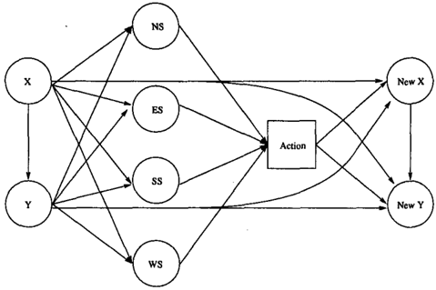
The problem of choosing an action can be represented by an influence diagram; the representation imposes a finite structure on the problem, namely that the agent is limited to a fixed number of actions. A single stage is shown in Figure 4. The four sensors are directly connected to the decision node. The two state variables affect the sen­ sors directly, but are themselves not directly observable by the agent. In principle, the single stage can be repeated any number of times; no-forgetting arcs connect the maze walker's previous sensors and actions to the the current ac­ tion. In the figure, the no-forgetting arcs have not been drawn.

The probabilistic inform a tion required by this influ­ ence diagram forms the agent model. Sensors can be modelled with the conditional probability distributions P(NSIX, Y), etc. Actuators can be modelled by the con­ ditional probability distributions P(N ewXIX, Y, Action) and P(N ewYIX, Y, Action, N ewY).

Four agent models were used in this test. These correspond to two sensor models: perfect and noisy; and two actuator models: perfect and noisy. The perfect sensors always de­ tect a wall when there is one, and never detect a wall when

there isn't one. The noisy sensor model has probability 0.9 that a wall is correctly detected, and 0.05 that a wall is de­ tected when no wall is there. The perfect actuators always put the agent in the correct square for a given action. The noisy actuator model depends on adjacent walls and obsta­ cles. The agent ends up in the right place for a given action with a probability of about 0.89, and with probability about 0.089, the agent fails to move. The noisy actuator has a very small probability (about 0.01) of moving to an incorrect ad­ jacent square.

The value function is not shown in the ID fragment. It de­ pends only on the position of the agent in the final stage, and puts full value ( 1.0) on being at the goal, and zero else­ where.

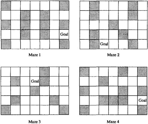
The mazes used in our experiments are shown in Figure 5 (Maze 1 is an example from [Littman, Cassandra, & Kael­ bling, 1995]). In our experiments, the agent is allowed ten stages to reach the goal, which makes it possible to reach the goal from each starting position. Using 10 stages, the tenth decision node has 49 direct predecessors.

Maze 1 has a simple policy which guides the perfect agent to the goal from each possible starting position. The policy guides the agent south whenever possible, or otherwise east whenever possible. If neither south nor east is possible, the agent moves west, if possible, and otherwise stays in place. This decision function is repeated for the first 8 stages. The final two steps of the policy direct the agent north one step and east one step. This policy has an expected value of 1.0, and can be represented by 8 decision trees which use 3 in­ ternal vertices each, followed by two decision trees which need no internal vertices.

Maze 2 has an ambiguity which cannot be resolved by fol­ lowing a path to the goal. An optimal policy can guide the perfect agent to the goal position from 24 of the 25 start­ ing positions of this maze, for a maximum expected value of 0.96. We estimate that an optimal policy for the perfect agent in this maze can be represented by 10 decision trees using a total of about 30 internal vertices.

We do not have optimal policies for Mazes 3 and 4, but all the ambiguities in these mazes can be resolved along a path to the goal, i. e., there exist policies which guide the perfect agent to the goal from all starting positions; these policies have expected value of 1.0. We estimate that the optimal policies can be represented by 10 decision trees using be­ tween 20 and 30 internal vertices in total.

The optimal policies for the agents with imperfect sensors or actuators are unknown; the value of the optimal policy depends in part on the difficulty of the maze.

3.2 THE RESULTS

The random access refinement algorithm was applied to these problems. The second best action heuristic was used to select leaf vertices to extend, and the maximal extension strategy was used to extend each leaf. The algorithm had 20 extensions in total allocated for each problem. Note that this resource limit excludes the optimal policy for all the mazes. The average run time on a SPARC Ultra-2 for these problems was 73 minutes.

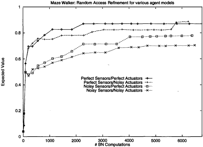
Figure 6 shows 4 datasets, corresponding to the variations of the agent model navigating Maze 1. The x -axis measures computational costs, in terms of the number of posterior probabilities and expected values computed (queries to the Bayesian network). The y-axis measures expected value of each policy. Each point on a curve represents the value of a policy in the sequence of policies constructed by the algo­ rithm. The first policy is the same for each of the problems, and represents the value of acting randomly before any de­ liberation has occurred.

For the perfect agent, the algorithm does not find the op­ timal policy using the allotted resources, but levels off at an expected value of 0.869565 after 2280 steps. The policy guides the agent to the goal from 20 of the 23 starting po­ sitions. This is roughly what one might expect, given that the optimal policy uses 24 internal vertices, and the algo­ rithm was given resources to include only 20 internal ver­ tices. The error here is 13% from optimal. We do not cur­ rently know whether the refinement process will find an op­ timal policy in reasonable time.

The curves in Figure 6 give an indication of how the con­ ditional probabilities underlying the agent model affect the performance profile. When the probabilities are very sharp, and a few states contain most of the probability mass (as in the case of the perfect agent), the increases tend to be steep

and plateaus are common. As the probability mass of is dis­ tributed over many more states (as in the agent with noisy sensors and noisy actuators), the increases tend to be less steep, and the plateaus shorter. These curves are typical.

Table 1 summarizes the performance of the various agents in the various mazes. The error for the perfect agent for all four mazes is 13%, 20%, 30% and 9%, respectively. For comparison, exhaustive enumeration would require more than 260 queries to compute complete policies. 2

For some of the agent models, the algorithm produces poli­ cies which decrease in value (for example, in the range of 0 to 500 queries in Figure 6). This behaviour is the result of making a local refinement when the commitment to the cur­ rent policy is weak. The refinement takes advantage of the relatively high probability of a non-MEV action. When the effects of the refinement are made global, the non-MEV ac­ tion drops in probability, and any action which was based on the non-MEV action will drop in value. This drop in value is temporary, and further refinement, stronger commitment, and global updates correct for the decrease.

The curve for the agent with noisy actuators and perfect sen­ sors also shows slight decreases in expected value in the range of 3500 to 5500 steps, followed by slight increases. This decrease has the same explanation as the more dra­ matic decreases observable earlier in the sequence. The ef-

2 To get an idea of the scale of this number: the figure is about 10 em wide; at this scale, 260 queries is approximately 15 light­ hours to the right. It would take about 23 billion years to compute according to the average reported above.

feet is smaller since the commitment to the MEV action is stronger.

Also of note is the fact that the algorithm is able to find a policy for the agent with noisy actuators and perfect sensors which exceeds the value of the best policy for the perfect agent. This behavior is due to the heuristics used by the al­ gorithm. In the case of the perfect agent, the heuristic chose to examine a certain set of contexts first. The noisy actua­ tors in the other agent gave a different heuristic value to the contexts.

Some of the variations on the Maze Walker have a rela­ tively large number of impossible information states; poli­ cies which summarize a large subspace of the information set can exploit these asymmetries, by not refining impossi­ ble contexts. Furthermore, if there is a subset of information states which cover most of the probability mass, it is possi­ ble to summarize a large portion of the state space by exam­ ining the most likely observations. Druzdzel [1994] argues that it is common for a few states to cover a large portion of the total probability mass in a joint probability distribu­ tion. Thus it seems reasonable to expect that policies which contain a small num b er of contexts will achieve fairly high value. The data presented in this paper support this expec­ tation.

Finally, it is important to acknowledge that the space ofiDs is very large, and the set of problems treated in this section is a small sample from a highly restricted subclass of IDs. The evidence in this section suggests that there exist large problems for which random access refinement can find poli-

Agent Model Sensor/Actuator	Best Policy	Steps
Perfect/Perfect	0.8696	2280
Perfect/Noisy	0.8874	6236
Noisy/Perfect	0.7767	6374
Noisy/Noisy	0.7045	6474

Maze 1

Agent Model Sensor/Actuator	Best Policy	Steps
Perfect/Perfect	0.7037	4522
Perfect/Noisy	0.5452	5581
Noisy/Perfect	0.6169	6079
Noisy/Noisy	0.4933	5799

Maze 3

Maze 2

Agent Model Sensor/Actuator	Best Policy	Steps
Perfect/Perfect	0.7692	4962
Perfect/Noisy	0.5159	5355
Noisy/Perfect	0.5887	5838
Noisy/Noisy	0.4703	5775

Maze 4

Agent Model Sensor/Actuator	Best Policy	Steps
Perfect/Perfect	0.9130	4564
Perfect/Noisy	0.6511	6219
Noisy/Perfect	0.6760	5319
Noisy/Noisy	0.6270	6162

Table 1: A summary of the best policies found by the random access refinement algorithm applied to several large decision problems. The optimal policy for the perfect agents is known to have expected value l.Ofor mazes 1, 3 and 4, and 0.96for maze 2. The optimal policy for these problems could be computed using dynamic programming, requiring about 260 steps.

cies which are reasonably valuable policies using reason­ able amounts of computational resources. These problems are too large to solve using traditional methods.

4 RELATED WORK

The information refinement approach is closely related to learning classification trees in machine learning (e.g., [Quinlan, 1986]). Heckerman et al. [1989] discusses an algorithm which constructs policies in a similar manner. Their interest is in representing a policy which can be used effectively by the decision maker on-line. The costs of building the decision tree are not taken into account; the costs of using the decision tree are compared to the cost of other on-line approaches.

Lehner and Sadigh [1993] also discusses the issue of com­ piling a decision problem into a situation-action tree. They do not emphasize computational cost; their goal is to take a complex problem and create rules for use by human de­ cision makers. They determine the best decision tree of a certain size, regardless of the cost of computing them.

Zhang & Boerlage [1995] simplify decision problems by removing inconsistent information states and "insignificant details" before constructing a policy for the problem. The significance of the details in the information state is mea­ sured in terms of the effects of the information state on the posterior probabilities of (unobservable) state variables.

Horvitz and Klein [1993] describe a decision theoretic ap­ proach to categorization based on utility. By aggregating states with similar utility values, and actions with similar values, decision models can be simplified for increased ef­ ficiency. Poh and Horvitz [1993] presents a greedy ap- proach to exploring how random variables in a decision model might be refined, i.e., how they can be given a more fine-grained set of values, to increase the utility of a deci­ sion. This work is intended to automate some of the effort that a decision analyst would put into reframing a decision problem, and deals with the refinement problem on a lower level than information refinement.

Information refinement is closely related to "input general­ ization" which is used to help deal with large state spaces in reinforcement learning. Chapman and Kaelbling [1991] adapt the Q-learning algorithm for large input spaces by us­ ing a decision tree in place of the table to represent the Q­ function. The decision tree is extended by "splitting" the function on significant input bits, as determined by tests for perceptual and value significance.

5 CONCLUSIONS

We have described an anytime algorithm for information refinement in multi-stage decision problems represented as influence diagrams. The process builds a stochastic deci­ sion tree for each decision node in the influence diagram. Each tree is initialized to be a single leaf labelled with the best action to perform without using any of the available in­ formation. A leaf is chosen heuristically, and is replaced with an extension. A probability distribution is imposed over the actions in the policy, which is a subjective assess­ ment of the probability that any particular action will be car­ ried out once the anytime refinement process is halted. The global effects of the refinement are propagated through the decision trees of the policy; probabilities are recomputed for decision trees following the refinement, and all leaf ver­ tices are recomputed in all the decision trees.

The procedure is very expensive asymptotically, and it is possible to construct an influence diagram for which the anytime algorithm will construct policies which are have no more than 50% of the expected value of the the optimal policy as long as no contexts are complete. An example of this kind of influence diagram has only uniform probability distributions and a value function in the form of the parity function on its inputs.

The results shown in this paper demonstrate that informa­ tion refinement constructs reasonably valuable policies for large decision problems using reasonable amounts of com­ putational resources. For some of the influence diagrams treated in this paper, no optimal policy is known. These problems are too large to enumerate the information space exhaustively.

Acknowledgements

The authors would like to thank the reviewers for helpful suggestions, and also Brent Boerlage of Norsys Software Corp. for advice and support in the use of the Netica API as our Bayesian network engine, and for many discussions. The second author is supported by the Institute for Robotics and Intelligent Systems, Project IC-7, and the National Sci­ ences and Engineering Council of Canada Operating Grant OGP0044121.

References

• [Chapman & Kaelbling, 1991] Chapman, D., and Kael­ bling, L. P. 1991. Input genelarization in delayed re­ inforcement learning: An algorithm and performance comparisons. In Proceedings of the TWelfth Interna­ tional Joint Conference on Artificial Intelligence, 726731.
• [Druzdzel, 1994] Druzdzel, M. J. 1994. Some proper­ ties of joint probability distributions. In Proceedings of the Tenth Conference on Uncertainty in Artificial Intelli­ gence, 187-194.
• [Heckerman, Breese, & Horvitz, 1989] Heckerman, D. E.; Breese, J. S.; and Horvitz, E. J. 1989. The compilation of decision models. In Uncertainty in Artificial Intelligence 5, 162-173.
• [Horsch & Poole, 1996] Horsch, M. C., and Poole, D. 1996. Flexible policy construction by information re­ finement. In Proceedings of the Twelfth Conference on Uncertainty in Artificial Intelligence, 315-324.
• [Horsch, 1998] Horsch, M. C. 1998. Flexible Policy Con­ struction by Information Refinement. Ph.D. Dissertation, Department of Computer Science, University of British Columbia. Forthcoming.
• [Horvitz & Klein, 1993) Horvitz, E. J., and Klein, A. C. 1993. Utility-based abstraction and categorization. In
• Proceedings of the Ninth Conference on Uncertainty in Artificial Intelligence, 128-135.
• [Howard & Matheson, 1984] Howard, R., and Matheson, J., eds. 1984. Readings on the Principles and Appli­ cations of Decision Analysis. CA: Strategic Decisions Group.
• [Lehner & Sadigh, 1993] Lehner, P. E., and Sadigh, A. 1993. Two procedures for compiling influence diagrams. In Proceedings of the Ninth Conference on Uncertainty in Artificial Intelligence, 335-341.
• [Littman, Cassandra, & Kaelbling, 1995] Littman, M. L.; Cassandra, A. R.; and Kaelbling, L. P. 1995. Learning policies for partially observable environments: Scaling up. In Proceedings of the Twelfth International Confer­ ence on MAchine Learning, 362-370.
• [Poh & Horvitz, 1993) Poh, K. L., and Horvitz, E. J. 1993. Reasoning about the value of decision-model refine­ ment: Methods and application. In Proceedings of the Ninth Conference on Uncertainty in Artificial Intelli­ gence, 174-182.
• [Qi & Poole, 1995] Qi, R., and Poole, D. 1995. New method for influence diagram evaluation. Computa­ tional Intelligence 11 (3):498-528.
• [Quinlan, 1986] Quinlan, J. 1986. Induction of decision trees. Machine Learning 1:81-106.
• [Shachter & Peot, 1992) Shachter, R., and Peot, M. 1992. Decision making using probabilistic inference methods. In Proceedings of the Eighth Conference on Uncertainty in Artificial Intelligence, 276-283.
• [Shachter, 1986) Shachter, R. D. 1986. Evaluating influ­ ence diagrams. Operations Research 34(6):871-882.
• [Smith, Holtzman, & Matheson, 1993) Smith, J. E.; Holtzman, S.; and Matheson, J. E. 1993. Structur­ ing conditional relationships in influence diagrams. Operations Research 41:280-297.
• [Zhang & Boerlage, 1995] Zhang, N. L., and Boerlage, B. 1995. Information filtering for planning in partially ob­ servable stochastic domains. Technical Report HKUST­ CS94-36, Department of Computer Science, Hong Kong University of Science and Technology.