Anytime State-Based Solution Methods for Decision Processes with non-Markovian Rewards

Sylvie Thiebaux

Computer Sciences Laboratory The Australian National University Canberra, ACT, Australia

Froduald Kabanza

Dept. Mathematiques et lnformatique Universite de Sherbrooke Sherbrooke, Quebec, Canada

Abstract

A popular approach to solving a decision pro­ cess with non-Markovian rewards (NMRDP) is to exploit a compact representation of the re­ ward function to automatically translate the NM­ RDP into an equivalent Markov decision pro­ cess (MOP) amenable to our favorite MOP so­ lution method. The contribution of this paper is a representation of non-Markovian reward func­ tions and a translation into MOP aimed at mak­ ing the best possible use of state-based any­ time algorithms as the solution method. By explicitly constructing and exploring only parts of the state space, these algorithms are able to trade computation time for policy quality, and have proven quite effective in dealing with large MOPs. Our representation extends future linear temporal logic (FLTL) to express rewards. Our translation has the effect of embedding model­ checking in the solution method. It results in an MOP of the minimal size achievable with­ out stepping outside the anytime framework, and consequently in better policies by the deadline.

1 INTRODUCTION

Markov decision processes (MOPs) are now widely ac­ cepted as the preferred model for decision-theoretic plan­ ning problems (Boutilier et a!., 1999). The fundamental as­ sumption behind the MOP formulation is that not only the system dynamics but also the reward function are Marko­ vian. Therefore, all information needed to determine the reward at a given state must be encoded in the state itself.

This requirement is not always easy to meet for plan­ ning problems, as many desirable behaviors are naturally expressed as properties of execution sequences, see e.g. (Drummond, 1989; Haddawy and Hanks, 1992; Bacchus and Kabanza, 1998; Pistore and Traverso, 2001 ). Typ­ ical cases include rewards for the maintenance of some property, for the periodic achievement of some goal, for the achievement of a goal within a given number of steps

John Slaney

Computer Sciences Laboratory The Australian National University Canberra, ACT, Australia

of the request being made, or even simply for the very first achievement of a goal which becomes irrelevant af­ terwards. A decision process in which rewards depend on the sequence of states passed through rather than merely on the current state is called a decision process with non­ Markovian rewards (NMRDP) (Bacchus et a!., 1996).

A difficulty with NMRDPs is that the most efficient MOP solution methods do not directly apply to them. The tradi­ tional way to circumvent this problem is to formulate the NMRDP as an equivalent MOP, whose states are those of the underlying system expanded to encode enough history­ dependent information to determine the rewards. Hand crafting such an expanded MDP (XMDP) can however be very difficult in general. This is exacerbated by the fact that the size of the XMDP impacts on the effectiveness of many solution methods. Therefore, there has been interest in automating the translation into an XMOP, starting from a natural specification of non-Markovian rewards and of the system's dynamics (Bacchus et al., 1996; Bacchus et al., 1997). This is the problem we focus on.

When solving NMRDPs in this setting, the central issue is to define a non-Markovian reward specification language and a translation into an XMOP adapted to the class of MOP solution methods and representations we would like to use for the type of problems at hand. The two previous proposals within this line of research both rely on past lin­ ear temporal logic (PLTL) formulae to specify the behav­ iors to be rewarded (Bacchus et al., 1996; Bacchus et a!., 1997), but adopt two very different translations adapted to two very different types of solution methods and represen­ tations. The translation in (Bacchus et a!., 1996) targets classical state-based solution methods such as policy iter­ ation (Howard, 1960) which generate complete policies at the cost of enumerating all states in the entire MOP, while that in (Bacchus et a!., 1997) targets structured solution methods and representations, which do not require explicit state enumeration, see e.g. (Boutilier et a!., 2000).

The aim of the present paper is to provide a language and a translation adapted to another class of solution methods which have proven quite effective in dealing with large MOPs, namely anytime state-based methods such as (Barto

et a!., 1995; Dean et a!., 1995; Thiebaux et a!., 1995; Hansen and Zilberstein, 200 I). These methods typically start with a compact representation of the MOP based on probabilistic planning operators, and search forward from an initial state, constructing new states by expanding the envelope of the policy as time permits. They may produce an approximate and even incomplete policy, but only ex­ plicitly construct and explore a fraction of the MDP. Nei­ ther of the two previous proposals is well-suited to such so­ lution methods, the first because the cost of the translation (most of which is performed prior to the solution phase) annihilates the benefits of anytime algorithms, and the sec­ ond because the size of the XMDP obtained is an obstacle to the applicability of state-based methods. Since here both the cost of the translation and the size of the XMDP it re­ sults in will severely impact on the quality of the policy obtainable by the deadline, we need an appropriate resolu­ tion of the tradeoff between the two.

Our approach has the following main features. The transla­ tion is entirely embedded in the anytime solution method, to which full control is given as to which parts of the XMDP will be explicitly constructed and explored. While the XMDP obtained is not minimal, it is of the minimal size achievable without stepping outside of the anytime frame­ work, i.e., without enumerating parts of the state or ex­ panded state spaces that the solution method would not nec­ essarily explore. This relaxed notion of minimality, which we call blind minimality is the most appropriate in the con­ text of anytime state-based solution methods.

When the rewarding behaviors are specified in PLTL, there does not appear to be a way of achieving a relaxed no­ tion of minimality as powerful as blind minimality with­ out a prohibitive translation. Therefore instead of PLTL, we adopt a variant of future linear temporal logic (FLTL) as our specification language, which we extend to handle rewards. While the language has a more complex seman­ tics than PLTL, it enables a natural translation into a blind­ minimal XMDP by simple progression of the reward for­ mulae. Moreover, search control knowledge expressed in FLTL (Bacchus and Kabanza, 2000) fits particularly nicely in this model- checking framework, and can be used to dra­ matically reduce the fraction of the search space explored by anytime solution methods.

The paper is organised as follows. Section 2 begins with background material on MOPs, NMRDPs, XMDPs, and anytime state-based solution methods. Section 3 describes our language for specifying non-Markovian rewards and the progression algorithm. Section 4 defines our translation into an XMDP along with the concept of blind minimal­ ity it achieves, and presents our approach to the embedded construction and solution of the XMDP. Finally, Section 5, provides a detailed comparison with previous approaches, and concludes with some remarks about future work. The proofs of the theorems appear in (Thiebaux et a!., 2002).

2 BACKGROUND

2.1 MDPs

A Markov decision process of the type we consider is a 5-tuple (S, so, A, Pr, R), where S is a finite set of fully ob­ servable states, so E S is the initial state, A is a finite set of actions (A( s) denotes the subset of actions applicable in s E S), {Pr(s,a,·) I sES,aEA(s)} is a family of proba­ bility distributions overS, such that Pr(s, a, s') is the prob­ ability of being in state s' after performing action a in state s, and R : S >-> 1R. is a reward function such that R( s) is the immediate reward for being in state s. It is well known that such an MOP can be compactly represented using prob­ abilistic extensions of traditional planning languages, see e.g., (Kushmerick et a!., 1995; Thiebaux et a!., 1995).

A stationary policy for an MOP is a function 1r : S >-> A, such that 1r( s) E A( s) is the action to be executed in state S. We note E( 1r) the envelope of the policy, that is the set of states that are reachable (with a non-zero probability) from the initial state so under the policy. If 1r is defined at all s E E ( 1r), we say that the policy is complete, and that it is incomplete otherwise. We note F ( 1r) the set of states in E( 1r) at which 1r is undefined. F( 1r) is called the fringe of the policy. We stipulate that the fringe states are absorbing. The value of a policy 1r at any state s E E( 1r), noted V,. ( s) is the sum of the expected rewards to be received at each future time step, discounted by how far into the future they occur. That is, for a non-fringe states E E(1r) \ F(1r):

where 0 :::; (3 :::; 1 is the discounting factor controlling the contribution of distant rewards. For a fringe state s E F( 1r ), V,. ( s) is heuristic or is the value at s of a complete default policy to be executed in absence of an explicit one. For the type ofMDP we consider, the value of a policy 1r is the value V,.(s0) of 1r at the initial state s0, and the larger this value, the better the policy.

2.2 STATE-BASED ANYTIME ALGORITHMS

Traditional state-based solution methods such as policy it­ eration (Howard, 1960) can be used to produce an optimal complete policy. Policy iteration can also be viewed as an anytime algorithm, which returns a complete policy whose value increases with computation time and converges to op­ timal. The main drawback of policy iteration is that it ex­ plicitly enumerates all states that are reachable from s0 in the entire MOP. Therefore, there has been interest in other anytime solution methods, which may produce incomplete policies, but only enumerate an increasing fraction of the states policy iteration requires.

For instance, (Dean et a!., 1995) describes methods which deploy policy iteration on judiciously chosen larger and

larger envelopes. Another example is (Thiebaux et al., 1995), in which a backtracking forward search in the space of (possibly incomplete) policies rooted at s0 is performed until interrupted, at which point the best policy found so far is returned. Real-time dynamic programming (RTDP) (Barto et al., 1995), is another popular anytime algorithm, which is to MDPs what learning real-time A* (Korf, 1990) is to deterministic domains. It can be run on-line, or off­ line for a given number of steps or until interrupted. A more recent example is the LAO* algorithm (Hansen and Zilberstein, 2001) which combines dynamic programming with heuristic search.

All these algorithms eventually converge to the optimal policy but need not necessarily explore the entire state space to guarantee optimality.1 When interrupted before convergence, they return a possibly incomplete but often useful policy. Another common point of these approaches is that they perform a forward search, starting from so and repeatedly expanding the envelope of the current policy one step forward. Since planning operators are used to com­ pactly represent the state space, these methods will only explicitly construct a subset of the MDP. In this paper, we will use these solution methods to solve decision processes with non-Markovian rewards which we define next.

2.3 NMRDPs AND EQUIVALENT XMDPs

We first need some notation. Let S* be the set of finite sequences of states over S, and sw be the set of possibly infinite state sequences. In the following, where 'f' stands for a possibly infinite state sequence in sw and i is a natural number, by T ; ' we mean the state of index i in f, by 'f ( i)' we mean the prefix (fo, . . . , fi) E S* of f, and by pre(f) we mean the set of finite prefixes of r. r 1; r 2 denotes the concatenation of f 1 E S* and f 2 E sw. For a dec\:>ion process D = (S,s0,A,Pr,R) and a state s E S, D(s) stands for the set of state sequences rooted at s that are feasible under the actions in D, that is: D( s) = {f E sw I fo = sand Vi :Ja E A(fi) Pr(ri, a, ri+1) > 0}. Note that the definition of D( s) does not depend on R and therefore also stands for NMRDPs which we describe now.

1 This is also true of the basic envelope expansion algorithm in (Dean eta!., 1995), under the same conditions as fo r LAO*.

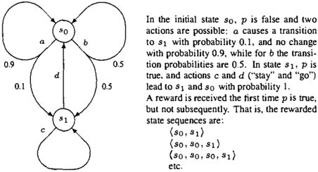
A decision process with non-Markovian rewards is identi­ cal to an MDP except that the domain of the reward func­ tion is S*. The idea is that if the process has passed through state sequence f(i) up to stage i, then the reward R(r(i)) is received at stage i. Figure 1 gives an example. Like the reward function, a policy for an NMRDP depends on his­ tory, and is a mapping from S* to A. As before, the value of policy 1r is the expectation of the discounted cumulative reward over an infinite horizon:

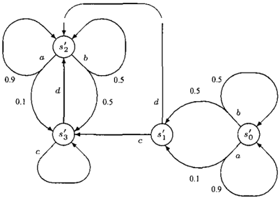
The clever algorithms developed to solve MDPs cannot be directly applied to NMRDPs. One way of dealing with this problem is to formulate the NMRDP as an equivalent MDP with an expanded state space (Bacchus et al., 1996). The expanded states in this XMDP (e-states, for short) augment the states of the NMRDP by encoding additional informa­ tion sufficient to make the reward history-independent. An e-state can be seen as labeled by a state of the NMRDP (via the function T in Definition 1 below) and by history information. The dynamics of NMRDPs being Markovian, the actions and their probabilistic effects in the XMDP are exactly those of the NMRDP. The following definition, adapted from (Bacchus et al., 1996), makes this concept of equivalent XMDP precise. Figure 2 gives an example.

Definition 1 MDP D'=\S', sb, A', Pr' , R') is an equivalent expansion (or XMDP)for NMRDP D = (S, so, A, Pr, R) if there exists a mapping T : S' >--> S such that:

1. r(sb) = so.
2. For all s' E S', A'(s') = A(r(s')).
3. For all s1, s2 E S, if there is a E A(s1) such that Pr(s1, a, s2) > 0, then for all sj E S' such that r(sD=s1. there exists a unique s2ES', r(s2)=s2, such that for alla E A'(sD, Pr'(sJ.,a,s2) = Pr(sJ,a,s2)·
4. For any feasible state sequence r E D(so) and f' E D'(sb) such that r(r;) = f d or all i, we have: R' (f;) = R(f( i)) for all i.

Items 1-3 ensure that there is a bijection between feasi­ ble state sequences in the NMRDP and feasible e-state se­ quences in the XMDP. Therefore, a stationary policy for the XMDP can be reinterpreted as a non-stationary policy for the NMRDP. Furthermore, item 4 ensures that the two poli­ cies have identical values, and that consequently, solving an NMRDP optimally reduces to producing an equivalent XMDP and solving it optimally (Bacchus et al., 1996):

Proposition 1 Let D be an NMRDP, D' an equivalent XMDP for it, and 1r1 a policy for D'. Let 7r be !_ he func­ tion defined on the sequence prefixes f(i) E D(so) by 1r(f( i)) = 1r'(f;), wherefor all j :'0 i r(fj) = r J · Then 1r is a policy forD such that V,.(so) = V,.. (sb).

When solving NMRDPs in this setting, the two key is­ sues are how to specify non-Markovian reward functions compactly, and how to exploit this compact representation to automatically translate an NMRDP into an equivalent XMDP amenable to our favorite solution methods. The goal of this paper is to provide a reward function specifica­ tion language and a translation that are adapted to the any­ time state-based solution methods previously mentioned. We take these problems in tum in the next two sections.

3 REWARDING BEHAVIORS

3.1 LANGUAGE AND SEMANTICS

Representing non-Markovian reward functions compactly reduces to compactly representing the behaviors of in­ terest, where by behavior we mean a set of fi­ nite sequences of states (a subset of S*), e.g. the { ( s0, s1 ) , ( so, so, s1 ) , ( s0, so, so, s1 ) . . . } in Figure 1. Re­ call that we get rewarded at the end of any prefix f( i) in that set. Once behaviors are compactly represented, it is straightforward to represent non-Markovian reward fimc­ tions as mappings from behaviors to real numbers - we shall defer looking at this until Section 3.5.

To represent behaviors compactly, we adopt a version of fu­ ture linear temporal logic (FLTL) augmented with a propo­ sitional constant ' $', intended to be read 'The behavior we want to reward has just happened' or 'The reward is re­ ceived now'. The language $FLTL begins with a set of basic propositions P giving rise to literals:

where T and j_ stand for 'true' and 'false', respectively. The connectives are classical 1\ and V, and the temporal modalities 0 (next) and U (weak until), giving formulae:

Because our 'until' is weak (!1 U h means h will be true from now on until h is, if ever), we can define the useful operator D (always): Of = f U j_ (f will always be true from now on). We also adopt the notations Ok f for k iter­ ations of the 0 modality (f will be true in exactly k steps), o9 f for the disjunction of o i for 1 :::: i :::: k (f will be true within the next k steps), and 09j for the conjunction ofO'f for 1::; i :S: k (f will be true at all the next k steps).

Although negation officially occurs only in literals, i.e., the formulae are in negation formal form (NNF), we allow our­ selves to write formulae involving it in the usual way, pro­ vided that they have an equivalent in NNF. Not every for­ mula has such an equivalent, because there is no such literal as · $ and because eventualities ('f will be true some time') are not expressible. These restrictions are deliberate.

The semantics of this language is similar to that of FLTL, with an important difference: unlike the interpretation of the propositional constants in P, which is fixed (i.e. each state is a fixed subset of P), the interpretation of the con­ stant $ is not. Remember that $ means 'The behavior we want to reward has just happened'. Therefore the interpre­ tation of $ depends on the behavior B we want to reward (whatever that is), and consequently the modelling relation f= stating whether a formula holds at the i-th stage of an arbitrary sequence f E sw, is indexed by B. Defining fs is the first step in our description of the semantics:

• ( f, i ) fs $ iff f ( i) E B
• (f,i) fs T
• (f, i) � j_
• (f, i) fs p, for pEP, iff p E fi
• (f , i) fs ·p, for p E P , iff p jtTi
• (r, i) Fs h 11 h iff (r, i) Fs h and (r, i) Fs h
• (r, i) Fs h v h iff (r, i) Fs h or (r, i) Fs h
• (f,i)fsOJ iff (f,i+l)�J
• (f,i) fs hUh iff Ilk 2': i if (llj, i::; j::; k (f,j) �h) then (r, k) � h

Note that except for subscript B and for the first rule, this is just the standard FLTL semantics, and that therefore $-free formulae keep their FLTL meaning. As with FLTL, we say r Fs f iff ( f,O) Fs J, and Fs f iffr Fs f for all r E sw.

The modelling relation I=; can be seen as specifying when a formula holds, on whic � reading it takes B as input. Our next and final step is to use the � relation to define, for a formula f, the behavior B f that 1 t represents, and for this we must rather assume that f holds, and then solve for B. For instance, let f be D(p -+ $), i.e., we get rewarded every time p is true. We would like B f to be the set of all finite sequences ending with a state containing p. For an arbitrary f, we take B f to be the set of prefixes that have to be rewarded if f is to hold in all sequences:

Definition 2 Bf = n{B I � f}

To understand Definition 2, recall that B contains prefixes at the end of which we get a reward and $ evaluates to true. Since f is supposed to describe the way rewards will be re­ ceived in an arbitrary sequence, we are interested in behav­ iors B which make $ true in such a way as to make f hold regardless of the sequence considered. However, there may be many behaviors with this property, so we take their inter­ section, 2 ensuring that B f will only reward a prefix if it has to because that prefix is in every behavior satisfying f. In all but pathological cases (see Section 3.3), this makes B f coincide with the (set-inclusion) minimal behavior B such that fi f. The reason for this 'stingy' semantics, making rewar !s minimal, is that f does not actually say that re­ wards are allocated to more prefixes than are required for its truth. For instance, D (p -> $) says only that a reward is given every time p is true, even though a more generous distribution of rewards would be consistent with it.

3.2 EXAMPLES

It is intuitively clear that many behaviors can be specified by means of $FLTL formulae. There is a list in (Bacchus et a!., 1996) of behaviors expressible in PLTL which it might be useful to reward. All of those examples are ex­ pressible naturally in $FLTL, as follows.

A simple example is the classical goal formula g saying that a goal pis rewarded whenever it happens: D(p -> $). As mentioned earlier, B 9 is the set of finite sequences of states such that p holds in the last state. If we only care that p is achieved once and get rewarded at each state from then on, we write D(p -> 0 $). The behavior that this for­ mula represents is the set of finite state sequences having at least one state in which p holds. By contrast, the formula -.p U (p 1\ $) stipulates that only the first occurrence of p is rewarded (i.e. it specifies the behavior in Figure I). To reward the occurrence of p at most once every k steps, we write D((ok+Ip 1\ -.o:;kp) _, ok+I$).

For response formulae, where the achievement of p is trig­ gered by the command c, we write D( c -> OD(p -> $)) to reward every state in which pis true following the first issue of the command. To reward only the first occurrence p after each command, we write D(c-> 0(-.p U (p 1\ $))). As for bounded variants for which we only reward goal achieve­ ment within k steps of the command, we write for example D(c-> O< k (P-> $)) to reward all such states in which p holds.

It is also worth noting how to express simple behaviors involving past tense operators. To stipulate a reward if p has always been true, we write $ U -.p. To say that we are rewarded if p has been true since q was, we write D(q-> ( $ U -.p)).

2 !f there is no B such that f1J J, which is the case for any $-free f which is not a logical theorem, then B 1 is n 0i.e. S*. This limiting case is a little artificial, but since such formulae do not describe the attribution of rewards, it does no harm.

3.3 REWARD NORMALITY

$FLTL is so expressive that it is possible to write formulae which describe "unnatural" allocations of rewards. For in­ stance, they may make rewards depend on future behaviors rather than on the past, or they may leave open a choice as to which of several behaviors is to be rewarded.3 An example of the former is Op -> $, which stipulates a re­ ward now if p is going to hold next. We call such formula reward-unstable. What a reward-stable f amounts to is that whether a particular prefix needs to be rewarded in order to make f true does not depend on the future of the sequence. An example of the latter is D (p -> $) V D ( -.p --+ $) which says we should either reward all achievements of the goal p or reward achievements of -.p but does not determine which. We call such forrnula reward-indeterminate. What a reward-determinate f amounts to is that the set of behav­ iors modelling f, i.e. {B I FE f}, has a unique minimum. If it does not, B f is insufficient (too small) to make f true.

In (Thiebaux et a!., 2002), we show that formulae that are both reward-stable and reward-determinate - we call them reward-normalare precisely those that capture the notion of"no funny business". This is this intuition that we ask the reader to note, as it will be needed in the rest of the paper. Just for reference then, we define:

Definition 3 f is reward-norrnal iff for every r E sw and every B <;; S* rfs f iff B f n pre(r) <;; B.

While reward-abnormal formulae may be interesting, for present purposes we restrict attention to reward-normal ones. Naturally, all formulae in Section 3.2 are norrnal.

3.4 $FLTL FORMULA PROGRESSION

Having defined a language to represent behaviors to be re­ warded, we now turn to the problem of computing, given a reward formula, a minimum allocation of rewards to states actually encountered in an execution sequence, in such a way as to satisfy the formula. Because we ultimately wish to use anytime solution methods which generate state se­ quences incrementally via forward search, this computa­ tion is best done on the fly, while the sequence is being generated. We therefore devise an incremental algorithm inspired from a model-checking technique normally used to check whether a state sequence is a model of an FLTL formula (Bacchus and Kabanza, 1998). This technique is known as formula progression because it 'progresses' or 'pushes' the formula through the sequence.

In essence, our progression algorithm computes the mod­ elling relation Js given in Section 3.1, but unlike the def-

3 These difficulties are inherent in the use of linear-time for­ malisms in contexts where the principle of directionality must be enforced. They are shared for instance by formalisms developed for reasoning about actions such as the Event Calculus and LTL action theories, see e.g. (Calvanese et al., 2002).

inition of Is , it is designed to be useful when states in the sequence become available one at a time, in that it de­ fers the evaluation of the part of the formula that refers to the future to the point where the next state becomes avail­ able. Let r; be a state, say the last state of the sequence prefix r( i) that has been generated so far, and let b be a boolean true iftT(i) is in the behavior B to be rewarded. The progression of the $FLTL formula f through r; given b, written Prog(b, f;, f), is a new formula satisfYing the following property. Where b <* (f( i) E B), we have:

That is, given that b tells us whether or not to reward f(i), f holds at f; iff the new formula Prog(b, f;,J) holds at the next (yet unavailable) state r i+ 1 in the sequence. The function Prog is defined below:

Algorithm 1 $FLTL Progression
Prog(true,s,$)	T
Prog(false,s,$)	_l
Prog(b,s, T)	T
Prog(b,s, _i)	_l
Prog(b,s,p)	T iffp E s and _l otherwise
Prog(b,s,•p)	T iffp f/ s and _l otherwise
Prog(b,s, !I 1\ h)	Prog(b,s, !I) 1\ Prog(b, s, h)
Prog(b,s, !IV h)	Prog(b,s, !I)V Prog(b,s, h)
Prog(b,s,Of)	f
Prog(b,s, !I U h)	Prog(b,s, h) V (Prog(b,s, !I) 1\ !I U h)
Rew(s,J)	true iffProg(false,s,f) = _l
$Prog(s,f)	Prog(Rew(s,f), s, f)

This is to be matched with the definition of Is in Sec­ tion 3 . I . Whenever Is evaluates a sub formula whose truth only depends on the current state, Prog does the same and return the formula T (resp. _i) accordingly. Whenever Is evaluates a subformula whose truth depends on future states, Prog defers the evaluation by returning a new sub­ formula to be evaluated in the next state. Note that Prog is computable in linear time in the length of f, and that for $-free formulae, it collapses to FLTL formula progression (Bacchus and Kabanza, 1998), regardless of the value of b.

Like Is , the function Prog assumes that B is known, but of course we only have f and one new state at a t ime of r, and what we really want to do is compute the appropriate B, namely that represented by f. So, similarly as in Section 3.1, we now turn to the second step, which is to use Prog to decide on the fly whether a newly generated sequence prefix r( i) is in B f and so should be allocated a reward. This amounts to incremen­ tally computing B f n pre(r), which provided f is reward normal, is the minimal behavior B such that (f, 0) Is f. We can do this as follows. According to Property 1,

(r, 0) Is f iff ( r, 1) Is Prog(bo, fo, fo), where fo = f and bo stands for r ( 0) E B. So B must be such that (f, 1) Is Prog(bo, fo, fo). To ensure minimality, we first assume that r ( O ) !/ B, i.e. b0 is false, and compute Prog(false, fo,Jo). If the result is _l, then since no mat­ ter what r 1 turns out to be (r, 1) F, _i, we know that the assumption about bo being false d � es not suffice to sat­ isfY f. The only way to get f to hold is to assign a re­ ward to r(O), so we take r(O) to be in B, i.e. b0 is true, and set the formula to be considered in the next state to h = Prog(true, fo,J0). If on the other hand the result is not _i, then we need not reward f(O) to make f hold, so we take r(o) not to be in B and seth = Prog(false, r0, f0).

When r 1 becomes available, we can iterate this reasoning to compute the smallest value of b1 such that (f, 1) Is h and that of the corresponding h = Prog(b1, r1, fi). And so on: progression through a sequence of states defines a sequence of booleans (b0, h, . . . ) and a sequence of formu­ lae (fo, JI, ... ). When f; becomes available, we can com­ pute the smallest value of b; such that ( r, i) Is f; and the corresponding fi+1· The value of b; represents f( i) E B f and tells us whether we should allocate a reward at that stage, while fi+ 1 is the new formula with which to iterate the process. In Algorithm 1, the function Rew takes r; and f; as parameter, and returns b; by computing the value of Prog(false, f;, f;). The function $Prog takes f; and f; as parameters and returns fi+1 by calling Prog(b;, f;, f;) with the value of b; is given by Rew(r;, f;).

The following theorem states that under weak assumptions, rewards are correctly allocated by progression:

Theorem 1 Let f be reward-norma/, and let (fo , JI , .. . ) be the result o f progressing it through the successive states o f a sequence r. Then, provided no f; is _i, for all i Rew(r;,f;) ifJf(i) E B1.

The premiss of the theorem is that f does not eventually progress to _l. Indeed if J; = _l for some i, it means that even rewarding r( i) does not suffice to make f true, so something must have gone wrong: at some earlier stage, the boolean b was made false where it should have been made true. The usual explanation is that the original f was not reward-normal. For instance Op -> $, which is reward unstable, progresses to _l in the next state if p is true there: regardless of r o, fo = Op -> $ = O·p V $, bo = false, and fi = ·p, so if p E f1 then h = _l. However, other (admittedly bizarre) possibilities exist: for example, although Op -> $ is reward-unstable, its substi­ tution instance OOT -> $,which also progresses to _lin a few steps, is logically equivalent to $ and is reward-normal.

If the progression method is to deliver the correct minimal behavior in all cases (even in all reward-normal cases) it has to backtrack on the choice of values for the b;s. In the inter­ est of efficiency, we choose not to allow backtracking. In­ stead, our algorithm raises an exception whenever a reward

formula progresses to ..L, and informs the user of the se­ quence which caused the problem. The onus is thus placed on the domain modeller to select sensible reward formulae so as avoid possible progression to ..L. It should be noted that in the worst ca�e, detecting reward-normality cannot be easier than the decision problem for $FLTL so it is not to be expected that there will be a simple syntactic criterion for reward-normality. In practice, however, commonsense precautions such as avoiding making rewards depend ex­ plicitly on future tense expressions suffice to keep things normal in all routine cases.

3.5 REWARD FUNCTIONS

With the language defined so far, we are able to compactly represent behaviors. The extension to a non-Markovian re­ ward function is straightforward. We represent such a func­ tion by a set ¢ c::;; $FLTL x lR of formulae associated with real valued rewards. We call ¢ a reward function specifi­ cation. Where formula f is a�sociated with reward r in ¢ , we write '(f : r) E ¢'. The rewards are a�sumed to be independent and additive, so that the reward function Rq, represented by ¢is given by:

E.g,if¢is {�pUp/\$: 5.2, D(q-> D$): 7.3}, we get a reward of 5.2 the first time that p holds, a reward of 7.3 from the first time that q holds onward�, a reward of 12.5 when both conditions are met, and 0 in otherwise.

Again, we can progress a reward function specification ¢ to compute the reward at all stages i of r. A� before, pro­ gression defines a sequence ( ¢0, ¢1, ... ) of reward function specifications, with ¢i+1 = SProg(f ;, ¢;),where SProg is the function that applies Frog to all formulae in a reward function specification:

Then, the total reward received at stage i is simply the sum of the real-valued rewards granted by the progression func­ tion to the behaviors represented by the formulae in ¢;:

By proceeding that way, we get the expected analog of The­ orem 1, which states progression correctly computes non­ Markovian reward functions:

Theorem 2 Let ¢ be a reward-norma f reward function specification, and let (¢0, ¢1 ... ) be the result of pro­ gressing it through the successive states of a sequence f. Then, provided ( ..L : r ) !f. ¢; for any i, then L {r I Rew(r;, f)}= Rq,(f(i)). (/or)E¢,

4We extend the definition of reward-normality to reward spec­ i fication functions the obvious way, by requiring that all reward formulae involved be reward normal.

4 SOLVING NMRDPs

4.1 TRANSLATION INTO XMDP

We now exploit the compact representation of a non­ Markovian reward function a� a reward function specifi­ cation to translate an NMRDP into an equivalent XMDP amenable to state-based anytime solution methods. Recall from Section 2.3 that each e-state in the XMDP is labeled by a state of the NMRDP and by history information suf­ ficient to determine the immediate reward. In the case of a compact representation a� a reward function specification ¢0, this addi tiona! information can be summarized by the progression of <Po through the sequence of states passed through. So an e-state will be of the form (s, ¢), where s E S is a state, and ¢ c::;; $FLTL x JR. is a reward function specification (obtained by progression). Two e-states (s, ¢) and (t, 1J;) are equal if s = t, the immediate reward� are the same, and the results of progressing ¢ and 1J; through s are semantically equivalent.

Definition 5 Let D = (S, so, A, Pr, R) be an NMRDP, and <Po be a reward function specification representing R (i.e., Rq,, = R, see Definition 4). We translateD into the XMDP D' = (S', s�, A', Pr', R') defined as follows:

Item I says that the e-states are labeled by a state and a reward function specification. Item 2 says that the initial e-state is labeled with the initial state and with the original reward function specification. Item 3 says that an action is applicable in an e-state if it is applicable in the state label­ ing it. Item 4 explains how successor e-states are and their probabilities are computed. Given an action a applicable in an e-state ( s, ¢), each successor e-state will be labeled by a successor state s' of s via a in the NMRDP and by the progression of ¢ through s. The probability of that e­ state is Pr( s, a, s') a� in the NMRDP. Note that the cost of computing Pr' is linear in that of computing Pr and in the sum of the lengths of the formulae in ¢. Item 5 has been motivated before (see Section 3.5).

It is ea�y to show that this translation lead� to an equivalent XMDP, a� defined in Definition 1. Obviously, the function r required for Definition! is given by r ( (s, ¢)) = s, and then the proof is a matter of checking conditions.

4.2 BLIND MINIMALITY

The size of the XMDP obtained, i.e. the number of e-states it contains is a key issue for us, as it has to be amenable to state-based solution methods. Ideally, we would like the XMDP to be of minimal size. However, we do not know of a method building the minimal equivalent XMDP incre­ mentally, adding parts as required by the solution method. And since in the worst case even the minimal XMDP can be larger than the NMRDP by a factor exponential in the length of the reward formulae (Bacchus et al., 1996), con­ structing it entirely would nullify the interest of anytime solution methods.

However, as we now explain, Definition 5 leads to an equiv­ alent XMDP exhibiting a relaxed notion of minimality, and which is amenable to incremental construction. By inspec­ tion, we may observe that wherever an e-state ( s, ¢) has a successor (s', ¢') via action a, this means that in order to succeed in rewarding the behaviors described in ¢ by means of execution sequences that start by going from s to s' via a, it is necessary that the future starting with s' suc­ ceeds in rewarding the behaviors described in ¢'. If ( s, ¢) i s i n the minimal equivalent XMDP, and if there really are such execution sequences succeeding in rewarding the be­ haviors described in¢, then (s', ¢') must also be in the min­ imal XMDP. That is, construction by progression can only introduce e-states which are a priori needed. Note that an e-state that is a priori needed may not really be needed: there may in fact be no execution sequence using the avail­ able actions that exhibits a given behavior. For instance, consider the response formula D(p...., O k q ...., O k $), i.e., every time command p is issued, we will be rewarded k steps later provided q is true then. Obviously, whether p is true at some stage affects the way future states should be rewarded. However, if k steps from there a state satisfying q can never be reached, then a posteriori p is irrelevant, and there was no need to label e-states differently according to whether p was true or not. To detect such cases, we would have to look perhaps quite deep into feasible futures. Hence the relaxed notion which we call blind minimality does not always coincide with absolute minimality.

We now formalise the difference between true and blind minimality. To simplify notation (avoiding functions like the T of Definition 1), we represent each e-state as a pair ( s, r) where s E S and r is a function from S* to R intu­ itively assigning rewards to sequences in the NMRDP start­ ing from s. A given s may be paired with several functions r corresponding to relevantly different histories of s. The XMDP is minimal if every such r is needed to distinguish between reward patterns in the feasible futures of s:

Theorem 3 Let S' be the set of e-states in a minimal equiv­ alent XMDP D' forD= (S, s0, A, Pr, R). Then for each e-state (s, r) E S' there exists a prefix f(i) E D(s0) such that fi = sand for all fl. E S*:

Blind minimality is similar, except that, since there is no looking ahead, no distinction can be drawn between feasi­ ble trajectories and others in the future of s:

Definition 6 Let S' be the set of e-states in an equivalent XMDP D' for an NMRDP D = (S, s0, A, Pr, R). D' is blind minimal iff for each e-state ( s, r) E S' there exists a prefix r( i) E D( So) such that r i = s and for all fl. E s·:

Theorem 4 Let D' be the translation of D as in Defini­ tion 5. D' is a blind minimal equivalent XMDP for D.

4.3 EMBEDDED SOLUTION/CONSTRUCTION

Blind minimality is essentially the best achievable with anytime state-based solution methods which typically ex­ tend their envelope one step forward without looking deeper into the future. Our translation into a blind-minimal XMDP can be trivially embedded in any of these solution methods. This will result in an 'on-line construction' of the XMDP: the method will entirely drive the construction of those parts of the XMDP which it feels the need to explore, and leave the others implicit. If time is short, a subopti­ mal or even incomplete policy may be returned, but only a fraction of the state and expanded state spaces will be constructed. Note that the solution method should raise an exception as soon as one of the reward formulae progresses to l., i.e., as soon as an expanded state (s, ¢) is built such that ( l. : r) E ¢, since this acts as a detector of unsuitable reward function specifications.

To the extent enabled by blind minimality, our approach al­ lows for a dynamic analysis of the reward formulae, much as in (Bacchus et al., 1997). Indeed, only the execution sequences realisable under a particular policy actually ex­ plored by the solution method contribute to the analysis of rewards for that policy. Specifically, the reward formulae generated by progression for a given policy are determined by the prefixes of the execution sequences realisable under this policy. This dynamic analysis is particularly useful, since relevance of reward formulae to particular policies (e.g. the optimal policy) cannot be detected a priori.

The forward-chaining planner TLPlan (Bacchus and Ka­ banza, 2000) introduced the idea of using FLTL to spec­ ify domain-specific search control knowledge and formula progression to prune unpromising sequential plans (plans violating this knowledge) from deterministic search spaces. This has been shown to provide enormous time gains, lead­ ing TLPlan to win the 2002 planning competition hand­ tailored track. Because our approach is based on progres­ sion, it provides an elegant way to exploit search control

一

knowledge, yet in the context of decision-theoretic plan­ ning. Here this results in a dramatic reduction of the frac­ tion of the XMDP to be constructed and explored, and therefore in substantially better policies by the deadline.

We achieve this as follows. We specify, via a $-free formula eo, properties which we know must be verified by paths fea­ sible under promising policies. Then we simply progress eo alongside the reward function specification, making e­ states triples (s, </>,c) where cis a $-free formula obtained by progression. To prevent the solution method to apply an action that leads to the control knowledge being violated, the action applicability condition (item 3 in Definition 5) becomes: a E A'((s,</>,c)) iff a E A(s) andc -#.l (the other changes are straightforward). For instance, the effect of the control knowledge formula D (p __, Oq) is to remove from consideration any feasible path in which p is not fol­ lowed by q. This is detected as soon as violation occurs, when the formula progresses to .l. Although this paper focuses on non-Markovian rewards rather than dynamics, it should be noted that $-free formulae can also be used to express non-Markovian constraints on the system's dynam­ ics, which can be incorporated in our approach exactly as we do for the control knowledge.

5 RELATED AND FUTURE WORK

It is evident that our thinking about solving NMRDPs and the use of temporal logic to represent them draws on (Bac­ chus et al., 1996). Both this paper and (Bacchus et al., 1997) advocate the use of PLTL over a finite past to spec­ ify non-Markovian rewards. In the PLTL style of specifi­ cation, we describe the past conditions under which we get rewarded now, while with $FLTL we describe the condi­ tions on the present and future under which future states will be rewarded. While the behaviors and rewards may be the same in each scheme, the naturalness of thinking in one style or the other depends on the case. Letting the kids have a strawberry dessert because they have been good all day fits naturally into a past-oriented account of rewards, whereas promising that they may watch a movie if they tidy their room (indeed, making sense of the whole notion of promising) goes more naturally with FLTL. One advantage of the PLTL formulation is that it trivially enforces the prin­ ciple that present rewards do not depend on future states. In $FLTL, this responsibility is placed on the domain mod­ eller. On the other hand, the greater expressive power of $FLTL opens the possibility of considering a richer class of decision processes, e.g. with uncertainty as to which rewards are received (the dessert or the movie) and when (some time next week, before it rains). This is a topic for future work. At any rate, as we now explain, $FLTL is bet­ ter suited than PLTL to solving NMRDPs using anytime state-based solution methods.

(Bacchus et al., 1996) proposes a method whereby an e­ state is labeled by a set of subformulae of the PLTL reward formulae. For the labeling, two extreme cases are consid­ ered: one very simple and the other elaborate. In the sim­ ple case, an e-state is labeled by the set of all subformu­ lae which are true at it. The computation of such simple labels can be done forward starting from the initial state, and so could be embedded in an anytime solution method. However, because the structure of the original reward for­ mulae is lost when considering subformulae individually, fine distinctions between histories are drawn which are to­ tally irrelevant to the reward function. Consequently, the expanded state space easily becomes exponentially bigger than the blind-minimal one. This is problematic with the solution methods we consider, because size severely affects their performance in solution quality.

In the elaborate case, a pre-processing phase uses PLTL formula regression to find sets of subformulae as poten­ tial labels for possible predecessor states, so that the sub­ sequent generation phase builds an XMDP representing all and only the histories which make a difference to the way actually feasible execution sequences should be rewarded. The XMDP produced is minimal, and so in the best case ex­ ponentially smaller than the blind-minimal one. However, the prohibitive cost of the pre-processing phase makes it unusable for anytime solution methods (it requires expo­ nential space and a number of iterations through the state space exponential in the size of the reward formulae). We do not consider that any method based on PLTL and regres­ sion will achieve a meaningful relaxed notion of minimality without a costly pre-processing phase. Our main contribu­ tion is an approach based on FLTL and progression which does precisely that, letting the solution method resolve the tradeoff between quality and cost in a principled way inter­ mediate between the two extreme suggestions above.

The structured representation and solution methods tar­ geted by (Bacchus et al., 1997) differ from the any­ time state-based solution methods our framework primar­ ily aims at, in particular in that they do not require explicit state enumeration at all (Boutilier et al., 2000; Hoey et al., 1999). Accordingly, the translation into XMDP given in (Bacchus et al., 1997) keeps the state and expanded state space implicit, and amounts to adding temporal variables to the problems together with the decision-tree describing their dynamics. It is very efficient but rather crude: the encoded history features do not even vary from one state to the next, which strongly compromises the minimality of the XMDP.5 However, non-minimality is not as problematic as with the state-based approaches, since structured solution methods do not enumerate states and are able to dynami­ cally ignore some of the variables that become irrelevant at some point of policy construction.

5 (Chomicki, 1995) uses a similar approach to extend a database with auxiliary relations containing additional informa­ tion sufficient to check temporal integrity constraints. As there is only ever one sequence of databases, what matters is more the size of these relations than avoiding making redundant distinctions.

In another sense, too, our work represents a middle way, combining the advantages conf erred by state-based and structured approaches, e.g. by (Bacchus et al., 1996) on one side, and (Bacchus et al., 1997) on the other. From the f ormer we inherit a meaningf ul notion of minimality. As with the latter, approximate solution methods can be used and can perf orm a restricted dynamic analysis of the reward formulae. In virtue of the size of the XMDP produced, the translation proposed in (Bacchus et al., 1997) is clearly unsuitable to anytime state-based methods. The question of the appropriateness of our translation to structured solu­ tion methods, however, cannot be settled as clearly. On the one hand, our approach does not preclude the exploitation of a structured representation of system 's states, 6 and f or­ mula progression enables even state-based methods to ex­ ploit some of the structure in '$FLTL space'. On the other hand, the gap between blind and true minimality indicates that progression alone is insufficient to always fully exploit that latter structure (reachability is not exploited). With our translation, even structured solution methods will not rem­ edy this. There is a hope that (Bacchus et al., 1997) is able to take advantage of the f ull structure of the reward func­ tion, but also a possibility that it will f ail to exploit even as much structure as our approach would, as efficiently.

The most important item f or future work is an empirical comparison of the three approaches in view to answering this question and identifying the domain f eatures f avor­ ing one over the other. Ours has been fully implemented as an extension (rewards, probabilities) of TLPlan's plan­ ning language (Bacchus and Kabanza, 2000), which, like TLPlan's, includes functions and bounded quantification. To allow for comparisons to be reported in a longuer ver­ sion of this paper, we are in the process of implementing the other two approaches, no implementation of either of them being reported in the literature. Another exciting future work area is the investigation of temporal logic f ormalisms for specif ying heuristics f or NMRDPs or more generally for search problems with temporally extended goals, as good heuristics are important to some of the solution meth­ ods we are targeting. Related to this is the problem of ex­ tending, to temporally extended goals, the GOALP predi­ cate (Bacchus and Kabanza, 2000) which is the key to the specification of reusable control knowledge in the case of reachability goals. Finally, we should investigate the pre­ cise relationship between our line of work and recent work on planning for weak temporally extended goals in non­ deterministic domains, such as attempted reachability and maintenance goals (Pistore and Traverso, 2002).

Acknowledgements Many thanks to Fahiem Bacchus, Rajeev Gore, Charles Grelton, David Price, Leonore Zuck, and reviewers for usef ul discussions and comments.

6Symbolic implementations of the solution methods we con­ sider, e.g. (Feng and Hansen, 2002), as well as formula progres­ sion in the context of symbolic state representations (Pistore and Traverso, 200 I ) could be investigated for that purpose.

References

• Bacchus, F., Boutilier, C., and Grove, A. ( 1 996). Rewarding be­ haviors. In Proc. AAAI-96, pages 1 1 60-1 1 67.
• Bacchus, F., Boutilier, C., and Grove, A. (1997). Structured so­ lution methods for non-markovian decision processes. In Proc. AAAI-97, pages 1 1 2-1 1 7.
• Bacchus, F. and Kabanza, F. ( 1 998). Planning for temporally ex­ tended goals. Annals o f M athematics and Artificial Intelli­ gence, 22:5-27.
• Bacchus, F. and Kabanza, F. (2000). Using temporal logic to ex­ press search control knowledge for planning. Artificial I n­ telligence, 1 1 6( 1 -2).
• Barto, A., Bardtke, S., and Singh, S. ( 1 995). Learning to act us­ ing real-time dynamic programming. Artificial Intelligence, 72:81-138.
• Boutilier, C., Dean, T ., and Hanks, S. ( 1 999). Decision-theoretic planning: Structural assumptions and computational lever­ age. In Journal o f Artificial Intelligence Research, vol­ ume I I , pages 1-94.
• Boutilier, C., Dearden, R., and Goldszmidt, M. (2000). Stochastic dynamic programming with factored representations. Artifi­ cial Intelligence, 1 2 1 ( 1 -2):49-107.
• Calvanese, D., De Giacomo, G., and Vardi, M. (2002). Reasoning about actions and planning in LTL action theories. In Proc. KR-02.
• Chomicki, J. (1 995). Efficient checking of temporal integrity con­ straints using bounded history encoding. ACM T ransactions on Database Systems, 1 0(2): 149-1 86.
• Dean, T., Kaelbling, L., Kinnan, J., and Nicholson, A. ( 1 995). Planning under time constraints in stochastic domains. Ar­ tificial I ntelligence, 76:35-74.
• Drummond, M. (1 989). Situated control rules. In Proc. KR-89, pages 103-1 13.
• Feng, Z. and Hansen, E. (2002). Symbolic LAO* search for fac­ tored markov decision processes. In Proc. AIPS-02 W ork­ shop on Planning via Model-Checking. To appear.
• Haddawy, P. and Hanks, S. ( 1 992). Representations for decision­ theoretic planning: Utility functions and deadline goals. In Proc. KR-92, pages 71-82.
• Hansen, E. and Zilberstein, S. (200 I). LAO*: A heuristic search algorithm that finds solutions with loops. Artificial Intelli­ gence, 1 29:35-62.
• Hoey, J., St-Aubin, R., Hu, A., and Boutilier, C. ( 1 999). SPUDD: stochastic planning using decision diagrams. In Proc. U AI99.
• Howard, R. (1960). Dynamic Programming and Markov Pro­ cesses. MIT Press, Cambridge, MA.
• Korf, R. (1 990). Real-time heuristic search. Artificial Intelligence, 42: 1 89-21 1 .
• Kushmerick, N., Hanks, S., and Weld, D. ( 1 995). An algorithm for probabilistic planning. Artificial Intelligence, 76:239286.
• Pistore, M. and Traverso, P . (200 I ). Planning as model-checking for extended goals in non-deterministic domains. In Proc. /JCAI-OI, pages 479-484.
• Pistore, M. and Traverso, P. (2002). Planning with a language for extended goals. In Proc. AAAI-02.
• Thiebaux, S., Hertzberg, J., Shoaff, W., and Schneider, M. ( 1 995). A stochastic model of actions and plans for anytime plan­ ning under uncertainty. International J ournal o f Intelligent S ystems, 1 0(2): 155-1 83.
• Thiebaux, S., Kabanza, F., and Slaney, J. (2002). A model­ checking approach to decision-theoretic planning with non-markovian rewards. Technical report, The Aus­ tralian National University, Computer Sciences Laboratory. http://csl.anu.edu.au/�thiebaux/papers/nmr.ps.gz.