Approximate inference on planar graphs using Loop Calculus and Belief Propagation

Vicen¸ c G´ omez

Hilbert J. Kappen

Department of Biophysics Radboud University Nijmegen 6525 EZ Nijmegen, The Netherlands

Michael Chertkov

Theoretical Division and Center for Nonlinear Studies Los Alamos National Laboratory Los Alamos, NM 87545

Editor:

[email protected] [email protected] [email protected]

Abstract

We introduce novel results for approximate inference on planar graphical models using the loop calculus framework. The loop calculus (Chertkov and Chernyak, 2006a) allows to express the exact partition function of a graphical model as a finite sum of terms that can be evaluated once the belief propagation (BP) solution is known. In general, full summation over all correction terms is intractable. We develop an algorithm for the approach presented in Chertkov et al. (2008) which represents an efficient truncation scheme on planar graphs and a new representation of the series in terms of Pfaffians of matrices. We analyze the performance of the algorithm for the partition function approximation for models with binary variables and pairwise interactions on grids and other planar graphs. We study in detail both the loop series and the equivalent Pfaffian series and show that the first term of the Pfaffian series for the general, intractable planar model, can provide very accurate approximations. The algorithm outperforms previous truncation schemes of the loop series and is competitive with other state-of-the-art methods for approximate inference.

Keywords: belief propagation, loop calculus, approximate inference, partition function, planar graphs.

1. Introduction

Graphical models are popular tools widely used in many areas which require modeling of uncertainty. They provide an effective approach through a compact representation of the joint probability distribution. The two most common types of graphical models are Bayesian Networks (BN) and Markov Random Fields (MRFs).

The partition function of a graphical model, which plays the role of normalization constant in a MRF or probability of evidence (likelihood) in a BN is a fundamental quantity which arises in many contexts such as hypothesis testing or parameter estimation. Exact computation of this quantity is only feasible when the graph is not too complex, or equiv-

c © Vicen¸ c G´ omez, Hilbert J. Kappen and Michael Chertkov.

alently, when its tree-width is small. Currently many methods are devoted to approximate this quantity.

The belief propagation (BP) algorithm (Pearl, 1988) is at the core of many of these approximate inference methods. Initially thought as an exact algorithm for tree graphs, it is widely used as an approximation method for loopy graphs (Murphy et al., 1999; Frey and MacKay, 1998). The exact partition function is explicitly related to the BP approximation through the loop calculus framework introduced by Chertkov and Chernyak (2006a). Loop calculus allows to express the exact partition function as a finite sum of terms (loop series) that can be evaluated once the BP solution is known. Each term maps uniquely to a subgraph, also denoted as a generalized loop, where the connectivity of any node within the subgraph is at least degree two. Summation of the entire loop series is a hard combinatorial task since the number of generalized loops is typically exponential in the size of the graph. However, different approximations can be obtained by considering different subsets of generalized loops in the graph.

It has been shown empirically (G´ omez et al., 2007; Chertkov and Chernyak, 2006b) that truncating this series may provide efficient corrections to the initial BP approximation. More precisely, whenever BP performs satisfactorily which occurs in the case of sufficiently weak interactions between variables or short-range influence of loops, accounting for only a small number of terms is sufficient to recover the exact result (G´ omez et al., 2007). On the other hand, for those cases where BP requires many iterations to converge, many terms of the series are required to improve substantially the approximation. A formal characterization of the classes of tractable problems via loop calculus still remains as an open question.

A step toward this goal has been done in Chertkov et al. (2008) where it was shown that for any graphical model, summation of a certain subset of terms can be mapped to a summation of weighted perfect matchings on an extended graph. For planar graphs (graphs that can be embedded into a plane without crossing edges), summation of the subset can be performed in polynomial time evaluating the Pfaffian of a skew-symmetric matrix associated with the extended graph. Furthermore, the full loop series can be expressed as a sum over certain Pfaffian terms, where each Pfaffian term accounts for a large number of loops and is solvable in polynomial time as well.

The approach of Chertkov et al. (2008) builds on classical results from 1960s by Kasteleyn (1963); Fisher (1966) and other physicists who addressed the question of counting the number of perfect matchings on a planar grid, also known as the dimer problem in the statistical physics literature (a dimer correspond to a colored edge of the graph, and a valid dimer configuration consists of exactly one dimer per any edge of the graph). The key result of Kasteleyn (1963); Fisher (1966) can be summarized as follows: the partition function of a planar graphical model defined in terms of binary variables can be mapped to a weighted perfect matching problem and calculated in polynomial time under the restriction that interactions only depend on agreement or disagreement between the signs of their variables. Such a model is known in statistical physics as the Ising model without external field . Notice that exact inference for a general binary graphical model on a planar graph (that is Ising model with external field) is intractable (Barahona, 1982).

Recently, some methods for inference over graphical models, based on the works of Kasteleyn and Fisher, have been introduced. Globerson and Jaakkola (2007) obtained upper bounds on the partition function for non-planar graphs with binary variables by decom-

position of the partition function into a weighted sum over partition functions of spanning tractable (zero field) planar models. The resulting problem is a convex optimization problem and, since exact inference can be done in each planar submodel, the bound can be calculated in polynomial time.

Another example is the work of Schraudolph and Kamenetsky (2008) which provides a framework for exact inference on a restricted class of planar graphs using the approach of Kasteleyn and Fisher. More precisely, they showed that any joint probability function defined on binary variables can be expressed in a functional form without external fields by adding a new auxiliary node linked to all the existing nodes. Under this transformation, single-variable external fields can be allowed for a subset B of variables. If the graphical model is Bouterplanar, which means that there exists a planar embedding in which the subset B of the nodes lie on the same face, the techniques of Kasteleyn and Fisher can still be applied.

Contrary to the two aforementioned approaches which rely on exact inference on a tractable planar model, the loop calculus directly leads to a framework for approximate inference on general planar graphs. Truncating the loop series according to Chertkov et al. (2008) already gives the exact result in the zero external field case. In the general planar case, however, this truncation may result into an accurate approximation that can be incrementally corrected by considering subsequent terms in the series.

In the next Section we review the main theoretical results of the loop calculus approach for planar graphs and introduce the proposed algorithm. In Section 3 we provide experimental results on approximation of the partition function for regular grids and other types of planar graphs. We focus on a planar-intractable binary model with symmetric pairwise interactions but nonzero single variable potentials. The source code used to derive these results is freely available at http://www.mbfys.ru.nl/staff/v.gomez/ . We end this manuscript with conclusions and future work in Section 4.

2. Belief Propagation and loop Series for Planar Graphs

We consider the Forney graph representation, also called general vertex model (Forney, 2001; Loeliger, 2004), of a probability distribution p ( σ ) defined over a vector σ of binary variables (vectors are denoted using bold symbols). Forney graphs are associated with general graphical models which subsume other factor graphs, e.g. those correspondent to BNs and MRFs. In Appendix A we show how to convert a factor graph model to its equivalent Forney graph representation.

A binary Forney graph G := ( V , E ) consists of a set of nodes V where each node a ∈ V represents an interaction and each edge ( a, b ) ∈ E represents a binary variable ab which take values σ ab := {± 1 } . We denote ¯ a the set of neighbors of node a . Interactions f a ( σ a ) are arbitrary functions defined over typically small subsets of variables where σ a is the vector of variables associated with node a , i.e. σ a := ( σ ab 1 , σ ab 2 , . . . ) where b i ∈ ¯ a .

The joint probability distribution of such a model factorizes as:

where Z is the normalization factor, also called the partition function.

From a variational perspective, a fixed point of the BP algorithm represents a stationary point of the Bethe 'free energy' approximation under proper constraints (Yedidia et al., 2000). In the Forney style notation:

where b a ( σ a ) and b ab ( σ ab ) are the beliefs (pseudo-marginals) associated to each node a ∈ V and variable ab . For graphs without loops, Equation (2) coincides with the Gibbs 'free energy' and therefore Z BP coincides with the exact partition function Z . If the graph contains loops, Z BP is just an approximation critically dependent on how strong the influence of the loops is.

We introduce now some convenient definitions related to the loop calculus framework.

Definition 1 A generalized loop in a graph G = 〈V , E〉 is any subgraph C = 〈 V ′ , E ′ 〉 , V ′ ⊆ V , E ′ ⊆ ( V ′ × V ′ ) ∩ E such that each node in V ′ has degree two or larger.

For simplicity, we will use the term 'loop', instead of 'generalized loop', in the rest of this manuscript. Loop calculus allows to represent Z explicitly in terms of the BP approximation via the loop series expansion:

where C is the set of all the loops within the graph. Each loop term r C is a product of terms µ a, ¯ a C associated with every node a of the loop. ¯ a C denotes the set of neighbors of a within the loop C :

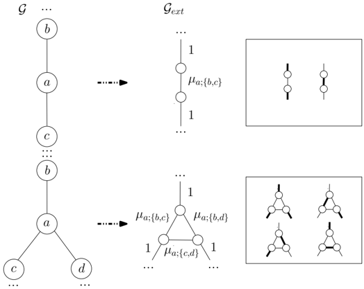
In this work we consider planar graphs where all nodes are of degree not larger than three, that is | ¯ a C | ≤ 3. We denote by triplet a node with degree three in the graph. In Appendix A we show that a graphical model can be converted to this representation at the cost of introducing auxiliary nodes.

Definition 2 A 2-regular loop is a loop in which all nodes have degree exactly two.

Definition 3 The 2-regular partition function Z ∅ is the truncated form of (3) which sums all 2 -regular loops only: 1

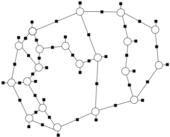
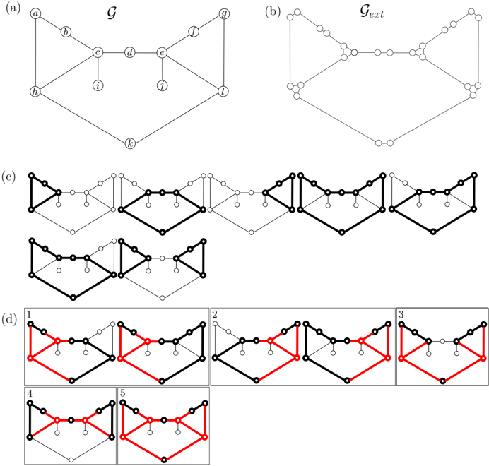
As an example, Figure 1a shows a small Forney graph and Figure 1c shows seven loops found in the corresponding 2-regular partition function.

2.1 Computing the 2 -regular Partition Function Using Perfect Matching

In Chertkov et al. (2008) it has been shown that computation of Z ∅ can be mapped to a dimer/matching problem, or equivalently, to the computation of the sum of all weighted perfect matchings within another graph. A perfect matching is a subset of edges such that

1. Notice that this part of the series was called single-connected partition function in Chertkov et al. (2008). Here we prefer to call it 2-regular partition function because loops with more than one connected component are also included in this part of the series.

each node neighbors exactly one edge from the subset. The weight of a matching is the product of weights of edges in the matching. The key idea of this mapping is to extend the original Forney graph G into an new graph G ext := ( V G ext , E G ext ) in such a way that each perfect matching in G ext corresponds to a 2-regular loop in G . (See Figures 1b and c for an illustration). Under the condition of planarity, the sum of all weighted perfect matchings can be calculated in a polynomial time following Kasteleyn's arguments. Here we reproduce these results with little variations and more emphasis on the algorithmic aspects.

Given a Forney graph G and the BP approximation, we simplify G and obtain the 2-core by removing nodes of degree one recursively. After this step, G is either the null graph (and then BP is exact) or it is only composed of vertices of degree two or three.

To construct the extended graph G ext we split each node in G according to the rules introduced by Fisher (1966) and illustrated in Figure 2. The procedure results in an extended graph of |V G ext | ≤ 3 |V| nodes and |E G ext | ≤ 3 |E| edges. It is easy to verify that each 2-regular loop in G is associated with a perfect matching in G ext and, furthermore, this correspondence is unique . Consider, for instance, the vertex of degree three in the bottom of Figure 2. Given a 2-regular loop C , vertex a can appear in four different configurations: either node a does not appear in C , or C contains one of the following three paths: b -a -c -, -b -a -d - or c -a -d -. These four cases correspond to node terms in a loop with values 1, µ a ; { b,c } , µ a ; { b,d } and µ a ; { c,d } respectively, and coincide with the matchings in G ext shown within the box on the bottom-right. An simpler argument applies to the vertex of degree two from the top portion of Figure 2.

Therefore, if we associate to each internal edge (new edge in G ext not in G ) of each split node a the corresponding term µ a ;¯ a C of Equation (4) and to the external edges (existing edges already in G ) weight 1, then the sum over all weighted perfect matchings defined on G ext is precisely z ∅ . The 2-regular partition function Z ∅ is obtained using Equation (5). Equivalently:

It is convenient that G ext is bi-connected, i.e. it has no articulation points. If needed, we add dummy edges with zero weight which do not alter the partition function or the original model.

Kasteleyn (1963) provided a method to compute this sum in polynomial time for planar graphs. We follow his approach. First, we create a planar embedding of G ext . A planar embedding of a graph divides the plane into disjoint regions that are bounded by sequences of edges in the graph. The regions are called faces . Second, we orient the edges of the planar embedding in such a way that for every face (except possibly the unbounded or external face) the number of clockwise oriented edges is odd. Algorithm 1 produces such an orientation (Karpinski and Rytter, 1998). It receives an undirected graph G ext and constructs a copy G ′ ext := ( V G ′ ext , E G ′ ext ) with properly oriented edges E G ′ ext .

Algorithm 1 Pfaffian orientation

Arguments: undirected bi-connected extended graph G ext .

• 2: Construct a spanning tree T of ¯ G ext .
• 1: Construct a planar embedding ¯ G ext of G ext .
• 3: Construct a graph H having vertices corresponding to the faces of G ext : Connect two vertices in H if the respective face boundaries share an edge not in T H is a tree. Root H to the external face.
• 4: G ′ ext := T .
• 6: for all face (vertex in H ) traversed in post-order do
• 5: Orient all edges in G ′ ext arbitrarily.
• 7: Add to G ′ ext the unique edge not in G ′ ext .
• 8: Orient it such that the number of clock-wise oriented edges is odd.
• 9: end for
• 10: RETURN directed bi-connected extended graph G ′ ext .

Finally, denote µ ij the weight of the edge between nodes i and j in G ′ ext . We create the following skew-symmetric matrix ˆ A = -ˆ A t :

 This matrix is known as the Tutte matrix of G ′ ext and the Pfaffian of ˆ A gives the desired sum up to the overall sign. The Pfaffian of ˆ A = ± √ Det( ˆ A ). However, z ∅ can be either positive or negative, and computing the value of the Pfaffian with the sign yet uncertain

• ¯

.

is not sufficient. Furthermore, since each element ˆ A ij can be negative not only due to the Pfaffian orientation but also if µ ij is negative, the sign of the Pfaffian needs to be corrected . This problem is fixed with the help of the original Kasteleyn's binary matrix:

If the sign of Pf( ˆ B ) is negative then the sign of Pf( ˆ A ) is changed. Notice that the absolute value of Pf( ˆ B ) coincides with the number of perfect matchings or the number of loops included in the sum if no additional edges have been added. The sign of Pf( ˆ B ) represents the correction. Therefore, the corrected value of z ∅ is:

Calculation of z ∅ can therefore be performed in time O ( N 3 ) where N is the number of nodes of G ext (Galbiati and Maffioli, 1994). For the special case of binary planar graphs with zero local fields the 2-regular partition function coincides with the exact partition function Z = Z ∅ = Z BP · z ∅ since the other terms in the loop series vanish.

2.2 Computing the Full Loop Series Using Perfect Matching

Chertkov et al. (2008) established that z ∅ is just the first term of a finite sum involving Pfaffians. We briefly reproduce their results here and provide an algorithm for computing the full loop series as a Pfaffian series.

Consider T defined as the set of all possible triplets (vertices with degree three in the original graph G ). For each possible subset Ψ ∈ T , including an even number of triplets, there exists a unique correspondence between loops in G including the triplets in Ψ and perfect matchings in another extended graph G ext Ψ constructed after removal of the triplets Ψ in G . Using this representation the full loop series can be represented as a Pfaffian series, where each term Z Ψ is tractable and is a product of the respective Pfaffian and the µ a ;¯ a terms associated with each triplet of Ψ: 2

The 2-regular partition function thus corresponds to Ψ = ∅ . We refer to the remaining terms of the series as higher order Pfaffian terms. Notice that matrices ˆ A Ψ and ˆ B Ψ depend on the removed triplets and therefore each z Ψ requires different matrices and different edge orientations. In addition, after removal of vertices in G the resulting graph may be disconnected. As before, in these cases we add dummy edges to G ext with zero weight to make the graph bi-connected again.

2. We omit the loop index in the triplet term µ a ;¯ a because nodes have at most degree three and therefore the set ¯ a always coincide in all loops which contain that triplet.

Figure 1d shows loops corresponding to the higher order Pfaffian terms on our illustrative example. The first and second subsets of triplets (d.1 and d.2) include summation over two loops whereas the remaining Pfaffian terms include uniquely one loop.

Exhaustive enumeration of all the subsets of triplets leads to a 2 |T | time algorithm, which is prohibitive. However, many triplet combinations may lead to forbidden configurations. Experimentally, we found that a principled way to look for higher order Pfaffian terms with large contribution is to search first for pairs of triplets, then groups of four, and so on. For large graphs, this also becomes intractable. Actually, the problem is very similar to the problem of selecting loop terms r C with largest contribution. The advantage of the Pfaffian representation, however, is that Z ∅ is always the Pfaffian term that accounts for the largest number of loop terms and is the most contributing term in the series. In this work we do not derive any heuristic for searching Pfaffian terms with larger contributions. Instead, in Section 3.1 we study the full Pfaffian series and subsequently we restrict ourselves on the accuracy of Z ∅ .

Algorithm 2 describes the full procedure to compute all terms using the representation of expression (6). The main loop of the algorithm can be interrupted at any time, thus leading to a sequence of algorithms producing corrections incrementally.

Algorithm 2 Pfaffian series
Arguments: Forney graph G
1: z := 0.
2: for	all (Ψ ∈ T ) do
3:	Build extended graph G ext Ψ applying rules of Figure 2.
4:	Set Pfaffian orientation in G ext Ψ according to Algorithm 1
5:	Build matrices ˆ A and ˆ B .
6:	Compute Pfaffian with sign correction z Ψ according to Equation (3).
7:	z := z + z Ψ ∏ a ∈ Ψ µ a ;¯ a .
8:	end for
9:	RETURN Z BP z

3. Experiments

In this Section we study numerically the proposed algorithm. To facilitate the evaluation and the comparison with other algorithms we focus on the binary Ising model, a particular case of the model (1) where factors only depend on the disagreement between two variables and take the form f a ( σ ab , σ ac ) = exp ( J a ; { ab,ac } σ ab σ ac ) . We consider also nonzero local potentials parametrized by f a ( σ ab ) = exp ( J a ; { ab } σ ab ) in all variables so that the model becomes planar-intractable.

We create different inference problems by choosing different interactions { J a ; { ab,ac } } and local field parameters { J a ; { ab } } . To generate them we draw independent samples from a Normal distribution { J a ; { ab,ac } } ∼ N (0 , β/ 2) and { J a ; { ab } } ∼ N (0 , β Θ), where Θ and β determine how difficult the inference problem is. Generally, for Θ = 0 the planar problem is tractable. For Θ > 0, small values of β result in weakly coupled variables (easy problems)

and large values of β in strongly coupled variables (hard problems). Larger values of Θ result in easier inference problems.

In the next Subsection we analyze the full Pfaffian series using a small example and compare it with the original representation based on the loop series. Next, we compare our algorithm with the following ones: 3

• Truncated Loop-Series for BP (TLSBP) (G´ omez et al., 2007), which accounts for a certain number of loops by performing depth-first-search on the factor graph and then merging the found loops iteratively. We adapted TSLBP as an any-time algorithm ( anyTLSBP ) such that the length of the loop is used as the only parameter instead of the two parameters S and M (see G´ omez et al. (2007) for details). This is equivalent to setting M = 0 and discard S . In this way, anyTLSBP does not compute all possible loops of a certain length (in particular, complex loops 4 are not included), but is more efficient than TLSBP.
• Cluster Variation Method ( CVM-Loopk ) A double-loop implementation of CVM (Heskes et al., 2003). This algorithm is a special case of generalized belief propagation (Yedidia et al., 2005) with convergence guarantees. We use as outer clusters all (maximal) factors together with loops of four (k=4) or six (k=6) variables in the factor graph.
• Tree-Structured Expectation Propagation ( TreeEP ) (Minka and Qi, 2004). This method performs exact inference on a base tree of the graphical model and approximates the other interactions. The method yields good results if the graphical model is very sparse.

When possible, we also compare with the following two variational methods which provide upper bounds on the partition function:

• Tree Reweighting ( TRW ) (Wainwright et al., 2005) which decomposes the parametrization of a probabilistic graphical model as a mixture of spanning trees of the model, and then uses the convexity of the partition function to get an upper bound.
• Planar graph decomposition ( PDC ) (Globerson and Jaakkola, 2007) which decomposes the parametrization of a probabilistic graphical model as a mixture of tractable planar graphs (with zero local field).

To evaluate the accuracy of the approximations we consider errors in Z and, when possible, computational cost as well. As shown in G´ omez et al. (2007), errors in Z , obtained from a truncated form of the loop series, are very similar to errors in single variable marginal probabilities, which can be obtained by conditioning over the variables under interest. We only consider tractable instances for which Z can be computed via the junction tree algorithm (Lauritzen and Spiegelhalter, 1988) using 8GB of memory. When studying the scalability of the approaches, we Given an approximation Z ′ of Z , the error measure used in this

3. We use the libDAI library (Mooij, 2008) for algorithms CVM-Loopk , TreeEP and TRW .

4. A complex loop is defined as a loop which can not be expressed as the union of two or more circuits or simple loops.

manuscript is:

As in G´ omez et al. (2007), we use four different message updates for BP: fixed and random sequential updates, parallel (or synchronous) updates, and residual belief propagation (RBP), a method proposed by Elidan et al. (2006) which selects the next message to be updated which has maximum residual , a quantity defined as an upper bound on the distance of the current messages from the fixed point. We report non-convergence when none of the previous methods converged. We report convergence at iteration t when the maximum absolute value of the updates of all the messages from iteration t -1 to t is smaller than a threshold ϑ = 10 -14 .

3.1 Full Pfaffian Series

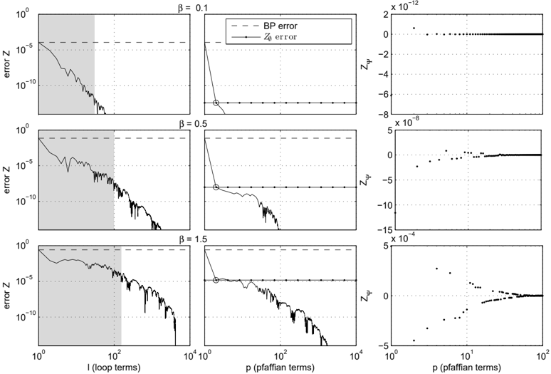
In the previous Section we have described two equivalent representations for the exact partition function in terms of the loop series and the Pfaffian series. Here we analyze numerically how these two representations differ using an example, shown in Figure 3 as a factor graph, for which all terms of both series can be computed. We analyze a single instance, parametrized using Θ = 0 . 1 and different pairwise interactions β ∈ { 0 . 1 , 0 . 5 , 1 . 5 } .

We use TLSBP to retrieve all loops, 8123 for this example, and Algorithm 2 to compute all Pfaffian terms. To compare the two approximations we sort all contributions, either loops or Pfaffians, by their absolute values in descending order, and then analyze how the errors are corrected as more terms are included in the approximation. We define partition functions for the truncated series in the following way:

Then Z TLSBP ( l ) accounts for the l most contributing loops and Z Pf ( p ) accounts for the p most contributing Pfaffian terms. In all cases, the Pfaffian term with largest absolute value Z Ψ 1 corresponds to z ∅ .

Figure 4 shows the error Z TLSBP (first column) and Z Pf (second column) for both representations. For weak interactions ( β = 0 . 1) BP converges fast and provides an accurate approximation with an error of order 10 -4 . Summation of less than 50 loop terms (top-left panel) is enough to obtain machine precision accuracy. Notice that the error is almost reduced totally with the z ∅ correction (top-middle panel). In this scenario, higher order terms of the Pfaffian series are negligible (top-right panel).

As we increase β , the quality of the BP approximation decreases. The number of loop corrections required to correct the BP error then increases. In this example, for intermediate interactions ( β = 0 . 5) the first Pfaffian term z ∅ improves considerably, more than five orders

of magnitude, on the BP error, whereas approximately 100 loop terms are required to achieve a similar correction (gray region of middle-left panel).

For strong interactions ( β = 1 . 5) BP converges after many iterations and gives a poor approximation. In this scenario also a larger proportion of loop terms (bottom-left panel) is necessary to correct the BP result up to machine precision. Looking at the bottom-left panel we find that approximately 200 loop terms are required to achieve the same correction as the one obtained by z ∅ . The z ∅ is quite accurate (bottom-middle panel).

As the right panels show, higher order Pfaffian contributions change progressively from a flat sequence of small terms to an alternating sequence of positive and negative terms which grow in absolute value as β increases. These oscillations are also present in the loop series expansion.

In general, we conclude that the z ∅ correction to the BP approximation can give a significant improvement even in hard problems for which BP converges after many iterations. Notice again that calculating z ∅ , the most contributing term in the Pfaffian series, does not require explicit search of loop or Pfaffian terms.

3.2 Grids

After analyzing the full Pfaffian series on a small random example we now restrict our attention to the Z ∅ approximation using Ising grids (nearest neighbor connectivity). First, we compare that approximation with other inference methods for different types of interactions (attractive or mixed) and then study the scalability of the method in the size of the graphs.

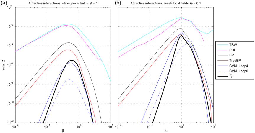
3.2.1 Attractive Interactions

We first focus on binary models with interactions that tend to align the neighboring variables to the same value, J a ; { ab,ac } > 0. If local fields are also positive J a ; { ab } > 0 , ∀ a ∈ V , Sudderth et al. (2008) showed that, under some additional condition, the BP approximation is a lower-bound of the exact partition function and all loops (and therefore Pfaffian terms too) have the same sign 5 . Although this is not formally proved for general models with attractive interactions regardless of the sign of the local fields, numerical results suggest that this property holds as well for this type of models.

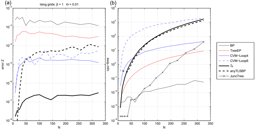
We generate grids with positive interactions and local fields, that is |{ J a ; bc }| ∼ N (0 , β/ 2) and |{ J a ; b }| ∼ N (0 , β Θ), and study the performance for various values of β , as well as for strong Θ = 1 and weak Θ = 0 . 1 local fields.

Figure 5 shows the average error over 50 instances reported by different methods. Using this setup, BP converged in all instances using sequential updates of the messages. The error curves of all methods show an initial growth and a subsequent decrease, a fact explained by the phase transition occurring in this model for Θ = 0 and β ≈ 1 (Mooij and Kappen, 2005). As the difference between the two plots suggest, errors are larger as Θ approaches zero. Notice, that Z ∅ = Z for the limit case of Θ = 0.

We observe that in all instances Z ∅ always improves over the BP approximation. Corrections are most significant for weak interactions β < 1 and strong local fields. For strong interactions β > 1 and weak local fields the improvement is less significant.

5. The condition is that all single variable beliefs at the BP fixed point must satisfy m ab = b ab (+1) -b ab ( -1) > 0 , ∀ ( a, b ) ∈ E

It appears that the Z ∅ approximation performs better than TreeEP in all cases except for very strong couplings, where they show very similar results. Interestingly, Z ∅ performs very similar to CVM-Loop4 which is known to be a very accurate approximation for this type of model, see Yedidia et al. (2000) for instance. We observe that in order to obtain better average results than Z ∅ using CVM, we need to select larger outer-clusters such as loops of length 6, which increases dramatically the computational cost.

The methods which provide upper bounds on Z (PDC and TRW) report the largest average error. PDC performs slightly better than TRW, as was shown in Globerson and Jaakkola (2007) for the case of mixed interactions. We remark that the worse performance of PDC for stronger couplings and weak local fields might be attributed to implementation artifacts, since for β > 4 we have numerical precision errors. In general, both upper bounds are significantly less tight than the lower bounds provided by BP and Z ∅ .

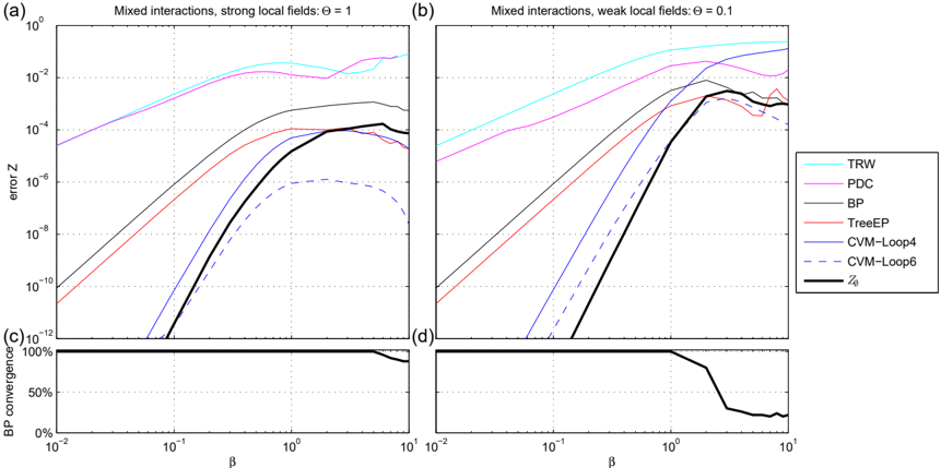
3.2.2 Mixed Interactions

We now analyze a more general Ising grid model where interactions and local fields can have mixed signs. In that case, Z BP and Z ∅ are no longer lower bounds on Z and loop terms can be positive or negative. Figure 6 shows results using this setup. Top panels show average errors and bottom panels show percent of instances in which BP converged using at least one of the methods described above.

For strong local fields (subplots a,c), we observe that Z ∅ improvements over BP results become less significant as β increases. It is important to note that Z ∅ always improves on the BP result, even when the couplings are very strong ( β = 10) and BP fails to converge for a small percentage of instances. Z ∅ performs slightly better than CVM-Loop4 and substantially better than TreeEP for small and intermediate β . All three methods show similar results for strong couplings β > 2. As in the case of attractive interactions, the best results are attained using CVM-loop6.

For the case of weak local fields (subplots b,d), BP fails to converge near the transition to the spin-glass phase. For β = 10, BP converges only in less than 25% of the instances. In the most difficult domain, β > 22, all methods under consideration give similar results (all comparable to BP). Moreover, it may happen that Z ∅ degrades the Z BP approximation because loops of alternating signs have major influence in the series. This result was also reported in G´ omez et al. (2007) when loop terms, instead of Pfaffian terms, where considered.

3.2.3 Scaling with Graph Size

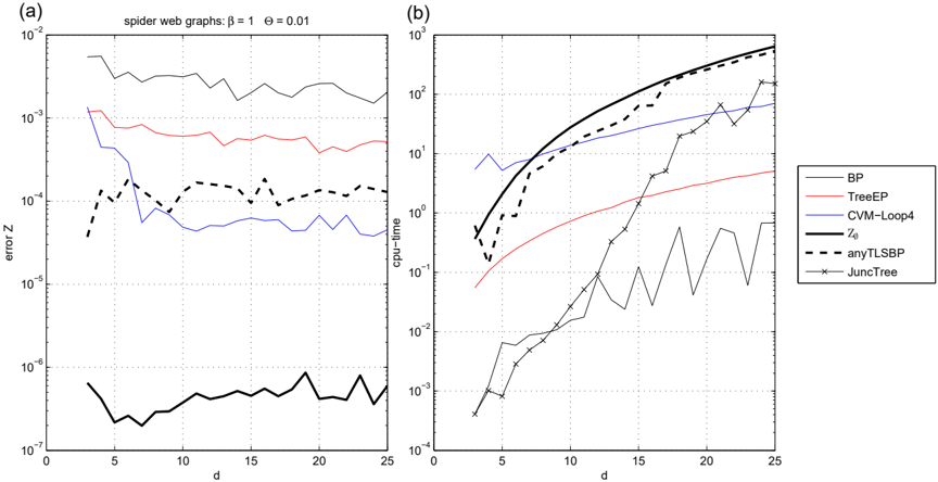
We now study how the accuracy of the Z ∅ approximation changes as we increase the size of the grid. We generate random grids with mixed couplings for √ N = { 4 , ..., 18 } and focus on a regime of very weak local fields Θ = 0 . 01 and strong couplings β = 1, a difficult

configuration according to the previous results. We compare Z ∅ also with anyTLSBP, a variant of our previous algorithm for truncating the loop series. We run anyTLSBP by selecting loops shorter than a given length, and the length is increased progressively. To provide a fair comparison between both methods, we run anyTLSBP for the same amount of cpu time as the one required to obtain Z ∅ .

Figure 7a shows the errors of different methods. Since variability in the errors is larger than before, we take the median for comparison. In order of increasing accuracy we get BP, TreeEP, anyTLSBP, CVM-Loop6, CVM-Loop4 and Z ∅ . We note that larger clusters in CVM does not necessarily result in better performance.

Overall, we can see that results are roughly independent of the network size N in almost all methods that we compare. The error of anyTLSBP starts being the smallest but soon increases because the proportion of loops captured decreases very fast. For N > 64, anyTLSBP performs worse than CVM. The Z ∅ correction, on the other hand, stays flat and we can conclude that it scales reasonably well. Interestingly, although Z ∅ and TLSBP use different ways to truncate the loop series, both methods show similar scaling behavior for large graphs.

Figure 7b shows the cpu time for all the tested approaches averaged over all cases. Concerning the approximate inference methods, in order of increasing cost, we have BP, TreeEP, CVM-Loop4, Z ∅ with anyTLSBP, and CVM-Loop6. Although the cpu time required to compute Z ∅ scales with O ( N 3 G ext ), its curve shows the steepest growth. We discuss how to correct this caveat in Section 4. The cpu time of the junction tree method quickly

increases with the tree-width of the graphs. For large enough N , exact solution via the junction tree method is no longer feasible because of its memory requirements. In contrast, for all approximate inference methods, memory demands do not represent a limitation.

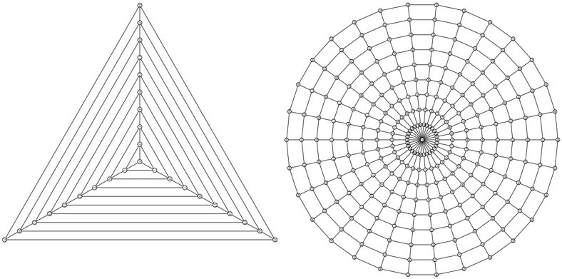
3.3 Radial grid graphs

In the previous subsection we analyzed the quality of the Z ∅ correction for graphs with a regular grid structure. Here, we carry over the analysis of the Z ∅ correction using planar graphs which consist of concentric polygons with a variable number of sides. Figure 8 illustrates these spider-web like graphs. We generate them as factor graphs with pairwise interactions which we subsequently convert to an equivalent Forney graph. (See Appendix A for details). Again, local field potentials are parametrized using Θ = 0 . 01 and interactions using β = 1. We analyze the error in Z as a function of the degree d of the central node.

Figure 9a shows the median of errors in Z of 50 random instances. First, we see that the variability of all methods, in particular anyTLSBP, is larger than in the regular grid scenario. Also, the improvement of CVM-Loop4 over BP is slightly less significant, possibly caused by the existence of the central node with a large degree. CVM-Loop6 does not converge for instances with d > 4 before 10 4 seconds and is not included in the analysis. We can say that all approaches present results independent of the degree d .

The Z ∅ approximation is the best method compared to the other tested approaches. The improvements of Z ∅ on CVM-Loop4 (the second best method) can be of more than two orders of magnitude and more than three orders of magnitude compared to BP.

Computational costs are shown in 9b. The best performance of Z ∅ comes at the cost of being the most expensive approximate inference approach for which we obtain results. Again, for larger graphs, exact solution via the junction tree is not feasible due to the large tree-width.

4. Discussion

We have presented an approximate algorithm based on the exact loop calculus framework for inference on planar graphical models defined in terms of binary variables. The proposed approach improves the estimate for the partition function provided by BP without an explicit search of loops.

The algorithm is illustrated on the example of ordered and disordered Ising model on a planar graph. Performance of the method is analyzed in terms of its dependence on the system size. The complexity of the partition function computation is exponential in the general case, unless the local fields are zero, when it becomes polynomial. We tested our algorithm on regular grids and planar graphs with different structures. Our experiments on regular grids show that significant improvements over BP are always obtained if single variable potentials (local magnetic fields) are sufficiently large. The quality of this correction degrades with decrease in the amplitude of external field, to become exact at zero external fields. This suggests that the difficulty of the inference task changes abruptly from very

easy, with no local fields, to very hard, with small local fields, and then decays again as external fields become larger.

The Z ∅ correction turns out to be competitive with other state of the art methods for approximate inference of the partition function. First of all, we showed that Z ∅ is much more accurate than upper bounds based methods such as TRW or PDC. This illustrates that such methods come at the cost of less accurate approximations. We have also shown that for the case of grids with attractive interactions, the lower bound provided by Z ∅ is the most accurate.

Secondly, we found that Z ∅ performs much better than treeEP for weak and intermediate couplings and shows competitive results for strong interactions. Concerning CVM, we showed that using larger outer clusters does not necessarily lead to better approximations. In general, the Z ∅ correction presented better results than CVM for our choice of regions.

Finally, we have presented a comparison of Z ∅ with TLSBP, which is another algorithm for the BP-based loop series using the loop length as truncation parameter. On the one hand, the calculation of Z ∅ involves a re-summation of many loop terms which in the case of TLSBP are summed individually. This consideration favors the Z ∅ approach. On the other hand, Z ∅ is restricted to the class of 2-regular loops whereas TLSBP also accounts for terms corresponding to more complex loop structures in which nodes can have degree larger than two. Overall, for planar graphs, we have shown evidence that the Z ∅ approach is better than TLSBP when the size of the graphs is not very small. We emphasize, however, that TLSBP can be applied to non-planar binary graphical models too.

Currently, the shortcoming of the presented approach is in its relatively costly implementation. However, since the bottleneck of the algorithm is the Pfaffian calculation and not the algorithm itself (used to obtain the extended graphs and the associated matrices), it is easy to devise more efficient methods than the one used here. Thus, one may substitute brute-force evaluation of the Pfaffians by a smarter one available for planar graphs. This reduces the cost from O ( N 3 ) to O ( N 3 / 2 ) (Galluccio et al., 2000; Loh and Carlson, 2006). Besides, the Pfaffian of ˆ B is binary, see Eq. (6), making it possible to improve using a bit-matrix representation (Schraudolph and Kamenetsky, 2008). Alternatively one could think of a strategy which does not require the Pfaffian of ˆ B . All these technical issues are the focus of our continuing investigation.

In this manuscript we have focused on inference problems defined on planar graphs with symmetric pairwise interactions and, to make the problems difficult, we have introduced local field potentials. Notice however, that the algorithm can also be used to solve models with more complex interactions, i.e. more than pairwise as in the case of the Ising model (see Chertkov et al., 2008, for a discussion of possible generalizations). This makes our approach more powerful than other approaches, namely, (Globerson and Jaakkola, 2007; Schraudolph and Kamenetsky, 2008), designed specifically for the pairwise interaction case.

Although planarity is a severe restriction, we emphasize that planar graphs appear in many contexts such as computer vision and image processing, magnetic and optical recording, or network routing and logistics. It would also be interesting (and possible) to consider extensions of the algorithm developed in the manuscript for approximate inference of some class of non-planar graphs. Thus, following the approach of Globerson and Jaakkola (2007), one can think of other types of spanning subgraphs more general than 'easy' planar graphs for which exact computation can be performed using perfect matching. The correction Z ∅

can be an accurate approximation for this spanning subgraphs and the resulting approximation method would also provide bounds on the exact result.

Acknowledgments

We acknowledge J. M. Mooij for providing the libDAI framework and A. Windsor for the planar graph functions of the boost graph library. We also thank V. Y. Chernyak, J. K. Johnson and N. Schraudolph for interesting discussions and A. Globerson for providing the Matlab sources of PDC. This research is part of the Interactive Collaborative Information Systems (ICIS) project, supported by the Dutch Ministry of Economic Affairs, grant BSIK03024. The work at LANL was carried out under the auspices of the National Nuclear Security Administration of the U.S. Department of Energy at Los Alamos National Laboratory under Contract No. DE-AC52-06NA25396.

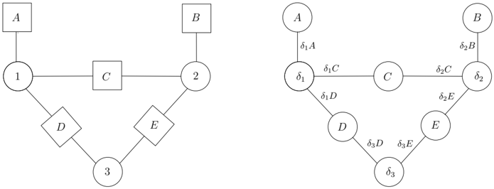
Appendix A: Converting a factor graph to a Forney Graph.

A probabilistic model is usually represented as a Bayesian Network or a Markov Random Field. Since bipartite factor graphs subsume both models, we show here how to convert a factor graph model defined in terms of binary variables to a more general Forney graph representation, for which the presented algorithm can be directly applied to.

On a bipartite factor graph G F = ( V F , E F ) the set V F is composed of a set of variable nodes I and a set of factor nodes J . Each variable node i ∈ I , i := { 1 , 2 , . . . } represents a variable which takes values σ i = {± 1 } . We label factor nodes using capital letters so that a = { A,B,... } , a ∈ J denotes a factor node which has an associated function f a ( σ a ) defined on a subset of variables ¯ a ∈ I . An (undirected) edge exists between two nodes ( a, i ) ∈ E F if i ∈ ¯ a .

Figure 10 shows an example of this transformation. Notice that, although we impose an direction in the edge labels, they remain undirected: ( δ i , a ) = ( a, δ i ), ∀ δ i , a ∈ V . For variables i ∈ V F which only appear in two factors, such as variable 3, the corresponding δ 3 node is redundant and can be removed. The joint distribution of G F is related to the joint distribution of G by:

Given G F , a direct way to obtain an equivalent Forney graph G is: first, to create a node δ i ∈ V for each variable node i ∈ V F , and second, to associate a new binary variable δ i a with values σ δ i a = {± 1 } to edges ( δ i , a ) ∈ E . Nodes δ i ∈ V are equivalent factor nodes denoting the characteristic function: δ i ( σ a ) = 1 if σ δ i a = σ δ i b , ∀ a, b ∈ ¯ δ i and zero otherwise. Finally, factor nodes c ∈ V F correspond to the same factor nodes c in V but defined in terms of the new variables δ i c , ∀ i ∈ ¯ c .

Once G has been generated following the previous procedure it may be the case that the nodes δ i ∈ V have degree three or larger. This happens if a variable i appears in more than

3 factor nodes on G F . It is easy to convert G to a graph were all δ i nodes have maximum degree three by introducing new auxiliary variables δ i 1 , δ i 2 , ... and new equivalent nodes. For instance, if variable i ∈ V F appears in 4 factors A,B,C,D :

Notice that although the models are equivalent, the number of loops in G may be larger than in G F . In the case that a factor in G F involves more than three variables, as sketched in Chertkov et al. (2008), one could split the node of degree N into auxiliary nodes of degree N -1 and compute Z ∅ on the transformed model. Alternatively, one can reduce the number of variables that enter a factor by clamping.

References

1. Barahona. On the computational complexity of Ising spin glass models. Journal of Physics A: Mathematical and General , 15(10):3241-3253, 1982. URL http://stacks.iop.org/0305-4470/15/3241 .
2. Chertkov and V. Y. Chernyak. Loop series for discrete statistical models on graphs. Journal of Statistical Mechanics: Theory and Experiment , 2006(06):P06009, 2006a.
3. Chertkov and V. Y. Chernyak. Loop calculus helps to improve Belief Propagation and linear programming decodings of LDPC codes. In invited talk at 44th Allerton Conference , September 2006b.
4. Chertkov, V. Y. Chernyak, and R. Teodorescu. Belief propagation and loop series on planar graphs. Journal of Statistical Mechanics: Theory and Experiment , 2008(05): P05003 (19pp), 2008. URL http://stacks.iop.org/1742-5468/2008/P05003 .
5. Elidan, I. McGraw, and D. Koller. Residual belief propagation: Informed scheduling for asynchronous message passing. In Proceedings of the 22nd Annual Conference on Uncertainty in Artificial Intelligence (UAI-06) , Boston, Massachussetts, July 2006. AUAI Press.

1. Fisher. On the dimer solution of the planar Ising model. Journal of Mathematical Physics , 7(10):1776-1781, 1966.
2. Jr. Forney, G.D. Codes on graphs: normal realizations. IEEE Transactions on Information Theory , 47(2):520-548, Feb 2001. ISSN 0018-9448. doi: 10.1109/18.910573.
3. J. Frey and D. J. C. MacKay. A revolution: belief propagation in graphs with cycles. In Advances in Neural Information Processing Systems 10 , pages 479-486, Cambridge, MA, 1998. MIT Press.
4. Galbiati and F. Maffioli. On the computation of Pfaffians. Discrete Applied Mathematics , 51(3):269-275, 1994. ISSN 0166-218X. doi: http://dx.doi.org/10.1016/0166-218X(92) 00034-J.
5. Galluccio, M. Loebl, and J. Vondr´ ak. New algorithm for the Ising problem: partition function for finite lattice graphs. Physical Review Letters , 84(26):5924-5927, Jun 2000. doi: 10.1103/PhysRevLett.84.5924.
6. Globerson and T. S. Jaakkola. Approximate inference using planar graph decomposition. In B. Sch¨ olkopf, J. Platt, and T. Hoffman, editors, Advances in Neural Information Processing Systems 19 , pages 473-480. MIT Press, Cambridge, MA, 2007.
7. G´ omez, J. M. Mooij, and H. J. Kappen. Truncating the loop series expansion for belief propagation. Journal of Machine Learning Research , 8:1987-2016, 2007. ISSN 1533-7928.
8. Heskes, K. Albers, and H. J. Kappen. Approximate inference and constrained optimization. In Proceedings of the 19th Annual conference on Uncertainty in Artificial Intelligence (UAI-03) , pages 313-320, San Francisco, CA, 2003. Morgan Kaufmann Publishers.
9. Karpinski and W. Rytter. Fast parallel algorithms for graph matching problems. pages 164-170. Oxford University Press, USA, 1998.
10. W. Kasteleyn. Dimer statistics and phase transitions. Journal of Mathematical Physics , 4(2):287-293, 1963. doi: 10.1063/1.1703953. URL http://link.aip.org/link/?JMP/4/287/1 .
11. L. Lauritzen and D. J. Spiegelhalter. Local computations with probabilities on graphical structures and their application to expert systems. Journal of the Royal Statistical society. Series B-Methodological , 50(2):154-227, 1988.
12. H.-A. Loeliger. An introduction to factor graphs. Signal Processing Magazine, IEEE , 21 (1):28-41, Jan. 2004. ISSN 1053-5888. doi: 10.1109/MSP.2004.1267047.
13. L. Loh and E. W. Carlson. Efficient algorithm for random-bond Ising models in 2d. Physical Review Letters , 97(22):227205, 2006. doi: 10.1103/PhysRevLett.97.227205. URL http://link.aps.org/abstract/PRL/v97/e227205 .
14. Minka and Y. Qi. Tree-structured approximations by expectation propagation. In Sebastian Thrun, Lawrence Saul, and Bernhard Sch¨ olkopf, editors, Advances in Neural Information Processing Systems 16 . MIT Press, Cambridge, MA, 2004.

1. M. Mooij. libDAI: A free/open source C++ library for discrete approximate inference methods, 2008. http://mloss.org/software/view/77/ .
2. M. Mooij and H. J. Kappen. On the properties of the Bethe approximation and loopy belief propagation on binary networks. Journal of Statistical Mechanics: Theory and Experiment , 2005(11):P11012, 2005.
3. P. Murphy, Y. Weiss, and M. I. Jordan. Loopy Belief Propagation for approximate inference: An empirical study. In Proceedings of the 15th Annual Conference on Uncertainty in Artificial Intelligence (UAI-99) , pages 467-475, San Francisco, CA, 1999. Morgan Kaufmann Publishers.
4. Pearl. Probabilistic Reasoning in Intelligent Systems: Networks of Plausible Inference . Morgan Kaufmann Publishers, San Francisco, CA, 1988. ISBN 1558604790.
5. Schraudolph and D. Kamenetsky. Efficient exact inference in planar Ising models. In Advances in Neural Information Processing Systems 22 . MIT Press, Cambridge, MA, 2008.
6. Sudderth, M. Wainwright, and A. Willsky. Loop series and Bethe variational bounds in attractive graphical models. In J.C. Platt, D. Koller, Y. Singer, and S. Roweis, editors, Advances in Neural Information Processing Systems 20 , pages 1425-1432. MIT Press, Cambridge, MA, 2008.
7. Wainwright, T. Jaakkola, and A. Willsky. A new class of upper bounds on the log partition function. IEEE Transactions on Information Theory , 51(7):2313-2335, July 2005.
8. S. Yedidia, W. T. Freeman, and Y. Weiss. Generalized belief propagation. In T.K. Leen, T.G. Dietterich, and V. Tresp, editors, Advances in Neural Information Processing Systems 13 , pages 689-695, December 2000.
9. S. Yedidia, W. T. Freeman, Y. Weiss, and A. L. Yuille. Constructing free-energy approximations and generalized belief propagation algorithms. IEEE Transactions on Information Theory , 51(7):2282-2312, July 2005.