Approximately Optimal Monitoring of Plan Preconditions

Craig Boutilier

Department of Computer Science University of Toronto Toronto, ON M5S 3H5 [email protected]

Abstract

Monitoring plan preconditions can allow for re­ planning when a precondition fails, generally far in advance of the point in the plan where the precondition is relevant. However, moni­ toring is generally costly, and some precondi­ tion failures have a very small impact on plan quality. We formulate a model for optimal pre­ condition monitoring, using partially-observable Markov decisions processes, and describe meth­ ods for solving this model effectively, though approximately. Specifically, we show that the single-precondition monitoring problem is gen­ erally tractable, and the multiple-precondition monitoring policies can be effectively approxi­ mated using single-precondition solutions.

1 Introduction

(e.g., a traffic jam may render a plan infeasible, but perhaps should not be taken into account if it occurs on a route that will not be reached for several hours). Even worse it does not factor in the cost of monitoring. Generally, precondition monitoring is not cost-free (e.g., tasking an agent to mon­ itor a route, or obtaining information from a Web source, has some cost). As a consequence, the value of monitoring a precondition from the time it is established until the time it is used may not be worth the cost (e.g., knowing about traffic many hours in advance is not likely to be much more useful than learning of it just before reaching the desired route, assuming a reasonable alternative route can be found at the later point in time). The second approach suffers from the opposite problem: though monitoring costs play no role, one cannot anticipate failures in advance. This generally means that the best repaired plan is not as good as one con­ structed when the failure is known in advance (e.g., if the traffic jam is not discovered until one is in it, the best re­ paired plan is likely of poor quality compared to one that avoided the j amm ed route entirely).

Uncertainty in planning problems is often handled by modeling the problem deterministically-enabling classi­ cal planning techniques to be used-but using methods for execution monitoring and replanning to handle situations that arise when the plan fails (e.g., when a precondition at some point fails to hold). Two extreme approaches can be adopted: The first requires monitoring all preconditions re­ quired by future actions in the plan (once they are estab­ lished); when one fails replanning is invoked. Refinements of this scheme are, of course, possible. 1 The second, and much more common, approach simply monitors the current state and should an unanticipated state be reached replan­ ning in invoked [8, 13, 7, 16, 2]. Variants of this scheme include the use of universal plans [ 14], essentially perform­ ing replanning in advance.

While both of these approaches have a certain appeal, they each have some rather serious drawbacks. The first ap­ proach allows one to anticipate precondition failures well in advance and replan as soon as one notices that the current plan will not work. However, it does not allow for the fact that precondition failure may be temporary or intermittent

1 For example, Veloso [ 16] monitors selected conditions for op­ portunities to construct better plans.

The decision of whether to monitor a plan precondition, and when to monitor it, involves balancing the cost of monitor­ ing and the value of monitoring information. Specifically, the value of a monitoring report at any point in time de­ pends on the odds that a report could change the plan, and the value of the best plan should that report not be received. As such, we can formulate the problem of monitoring as a partially-observable Markov decision process (POMDP). To do so requires that we have available the following in­ formation prior to plan execution time:

• the probability that preconditions may fail
• the cost of attempting to execute a plan action when its precondition has failed
• the value of the best alternative plan at any point dur­ ing plan execution (i.e., given that we abandon the cur­ rent plan at that point)
• a model of monitoring processes and their accuracy (e.g., the probability that a precondition is reported to be OK when it has in fact failed).

We assume that such information can be obtained or esti­ mated, and discuss these assumptions further below.

Unfortunately, though optimal monitoring can be formu­ lated as a POMDP, for any nontrivial plan, the size of the required POMDP takes it far from the realm of practical solution. Plans of only three steps (and three precondi­ tions) severely tax state-of-the-art algorithms. For this rea­ son we propose a class of heuristic techniques for solv­ ing the optimal monitoring problem. These methods in­ volve solving the monitoring problem for individual pre­ conditions, then constructing an (online) monitoring policy based on these component solutions. Though the individual problems also involve solving POMDPs, these remain very small and tractable. Thus the construction of monitoring policies for plans involving hundreds of steps is rendered feasible using our heuristic methods. We demonstrate em­ pirically on a small selection of problems that the solution quality of our techniques is generally quite good.

The main contributions of this work are twofold. We first provide a decision-theoretic model of plan monitoring. This model makes clear the role that value of information plays in optimal plan monitoring and the sequential nature of the decision problem. Neither of these characteristics is present in the existing plan-monitoring literature. The sec­ ond contribution is a tractable class of methods for solv­ ing the plan monitoring problem. Though these methods are heuristic and we currently explore their quality empir­ ically, we expect that they should yield to theoretical er­ ror analysis. These algorithms make the abstract monitor­ ing problem computationally manageable, thus making our decision-theoretic model a practical alternative to standard classical plan-monitoring methods.

2 The Plan Monitoring Problem

Classical planning techniques have advanced to the point where large planning problems involving hundreds of ac­ tions in sophisticated domains (e.g., logistics, process plan­ ning) can be solved effectively. However, these models in­ variably assume away uncertainty, modeling problems de­ terministically. Even though this modeling assumption may be reasonable, uncertainty (e.g., in action effects, or exoge­ nous events) must be dealt with when it impacts the ability to execute the plan. Plan and execution monitoring and re­ planning are often used in the regard.

The simplest monitoring model involves monitoring the es­ tablished preconditions of every action at each point in time until that action is executed. If a precondition has failed (e.g., due to unanticipated exogenous events) then we re­ plan from the current point in the plan subject to the ob­ served constraints. Unfortunately, despite offering opti­ mal object-level performance, this model may be too costly to implement. If precondition monitoring has some cost, the expected benefit in terms of improved object-level (re­ paired) plan quality may not outweigh the monitoring costs. Furthermore, if the monitoring reports are subject to error (e.g., unreliable Web sources, or faulty sensors), this ap­ proach is not satisfactory. A more refined decision-theoretic model is required, one where the probability of precondition failure and the cost of precondition monitoring are balanced against the expected improvement in plan quality offered

by timely information about the status of that precondition. This allows one to optimally decide if and when to monitor a given precondition. In this section, we formulate a specific version of the plan monitoring problem and describe how it can be solved optimally when cast as a POMDP.

It is important to note that a planning problem where pre­ condition failure and monitoring are both possible can be directly posed and solved as a POMDP. Specifically, assum­ ing the availability of the information required for optimal plan monitoring (e.g., precondition failure probabilities and monitoring accuracy models), a POMDP for the planning problem-as opposed to the plan monitoring problem--can be formulated readily. Forcing the problem into a classi­ cal framework, even with good execution monitoring and replanning strategies, will generally lead to suboptimal be­ havior. Despite this, breaking up the problem by construct­ ing a classical plan together with a monitoring policy can prove fruitful for several reasons. Most importantly, the POMDP formulation will generally prove impossible to solve for all but the most trivial problems. As such, the clas­ sical model can be viewed as a way of approximating the solution of the underlying POMDP. This isn't to say that other ways of approximating the POMDP's solution would not also be appropriate; and there has been little if any re­ search on how to directly form a deterministic relaxation of a POMDP or bound the quality of the classical plans so formed. But this form of solution has the advantage of rely­ ing on widely-used (and often very efficient) classical plan­ ning technology. Apart from this, the monitoring model we propose can be used with any classical plan, regardless of how it was constructed (e.g., it may simply be a plan con­ structed by a human expert). Since the classical view of plans as sequences of actions is often very natural in many domains, plan monitoring remains an important problem to be tackled using decision-theoretic techniques.

2.1 A Motivating Example

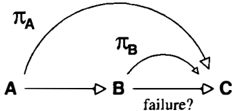
To illustrate the types of tradeoffs that must be addressed in plan monitoring, consider the following simple route plan­ ning example, illustrated in Figure 1. The best (e.g., lowest cost) plan 1r to reach goal location C from initial location A traverses the bottom-most links through location B. We in­ formally say that action A moves from A to B, thus the plan consists of two actions, A and B. If the link B --+ C fails (e.g., become impassable), the best plan from A involves an alternative route 7rA, and similarly the best plan from B is 1r B. We can monitor this link at any point in time for a cer­ tain cost, say, just before execution of A or B. If we learn that a link has failed, we can adopt the best alternative plan for the point at which failure was discovered.

Intuitively, one should monitor the link B -t C at some point if the expected value of information (EVOI) obtained by monitoring outweighs the cost of obtaining that informa­ tion. For example, suppose we monitor B -t C just prior to execution of action B. If we learn of link failure, the best "repaired" plan 7rB has value v( 7rB ) . If we had not learned of this failure, we would have continued execution of the original plan 1r, with a failure occurring when we try to ex­ ecute B. We assume that this failure will be repaired when it occurs, giving us an plan with value v( 'Trfai d · Therefore, the value of learning of link failure at point B is given by v( 7rB ) -v( 1r Jail ) . 2 EVOI is given by

where Pr(B) is the probability of link failure occurring by "time" B. Monitoring just prior to B is then worthwhile if the EVOI is greater than the monitoring cost.

We will develop a model below that makes precisely these tradeoffs. However, there are a number of subtleties that must be dealt with to provide an accurate account. First, as presented above, we have assumed that peifect informa­ tion is available, when, in fact, monitoring information is likely to be error-prone or uninformative. To deal with this we assume the existence of "sensor models" that describe the probability that a monitoring report is faulty in various ways. This also requires that we maintain a belief state de­ scribing the probability of precondition failures based on previous monitoring reports; we will seldom know of fail­ ure with certainty. We must also account for the sequential nature of the problem. Applying this reasoning to monitor­ ing prior to action A might suggest that monitoring at that point is also useful. But, in fact, this decision depends on whether one should monitor at point B. If it is worthwhile monitoring at B, it may not be worthwhile to additionally monitor at A. Intuitively, if v( 7rB ) is close to v( 1r A), then monitoring at A is probably not worthwhile, while if v( 1r A) is much greater, it probably is. The sequential nature of the problem demands a dynamic programming formulation of monitoring policy construction.

2.2 Modeling Assumptions

We assume that we have a deterministic planning problem, which has been solved with a classical plan 1r; this is a sequence of (deterministic) actions ( at, a2, · · · , a n ) . We somewhat loosely use the term time t to refer to the point just prior to the execution of at (thus time ranges from 1 to n + 1). The preconditions for action at all hold at timet in normal plan execution. For simplicity we assume each ac­ tion has a single precondition; thus we use the terms "mon­ itoring an action" and "monitoring a precondition" inter­ changeably.

In general, preconditions should only be considered for monitoring at certain points in the plan. The monitoring in­ terval for at is the interval between the establishment of the precondition of at and time t. 3 There is no point consider­ ing the monitoring of at outside of this interval. Again for

2We require that v ( 7rB ) 2:: v ( 11'Jail ) since one could always ignore failure if it is discovered.

3 A precondition p for at is established by action a i, j < t,

expository purposes, we assume that relevant preconditions have been established prior to the execution of the plan; that is, no action at establishes the (monitored) precondition for a future action at+k. This is merely to keep notation to a minimum-the techniques that follow make no important use of this fact.

We assume a plan value or cost model: for any alternative plan 1r', we know the value v(1r') of that plan. This may, for instance, simply ascribe higher value to plans with lower total action cost. Apart from knowing v ( 1r) for the original plan 1r, we also assume that we can determine by planning, or estimate by some other means, the value of the best alter­ native plans at each timet. Specifically, if we know that the precondition for ak E 1r has failed, the best alternative plan 'Tr j is known-or at least some estimate of its value v( 'Trj ) ­ for each 1 :::; j :::; k. So if we abandon 1r at time j because some future precondition has failed, the best alternative has a known value. We also know the value of attempting to execute an action in the original plan when its precondition does not hold, and subsequently implementing the best re­ paired plan. We dub this plan 1r£. (If the truth of precon­ ditions can't be unknown before an action is attempted, we simply need to set 1r£ = 'Trk.)

Though actions are modeled as though they have determin­ istic effects, certain exogenous events can occur that de­ stroy established preconditions. In order to construct op­ timal monitoring strategies, we must have some model of the likelihood of precondition failure. We adopt a general model of exogenous events, using a spontaneous transi­ tion model T(s'i s), where s and s' denote arbitrary system states. The quantity T( s'i s) denotes the probability that the system state s will transition to state s' due to the occurrence of some exogenous event (or events).4 From the point of view of plan monitoring, we are interested only in precon­ dition failure, so the required state space S simply consists of all truth assignments to plan preconditions. 5 To ease the modeling burden, we adopt the assumption of precondition failure independence, requiring that the probability of one precondition changing its state is independent of any other. Thus we can model transitions using n 2 x 2 transition ma­ trices, where Ti denotes the dynamics of the jth precondi­ tion. Specifically, Ti ( · PIP ) denotes the probability of pre­ condition failure, while Ti (p I · P) denotes the probability of spontaneous precondition repair (e.g., clearing of a traffic jam). Dealing with complex events that induce correlations in the failures of different preconditions can be modeled in probabilistic STRIPS notation [9, 10], dynamic Bayes nets [6, 3], or other representations. We need not move to full 2n x 2n transition matrices.

A set of monitoring actions M is assumed, each action pro-

if ai makes p true and no intervening action ak, j < k < t af­ fects p. If no such a i makes p true, it is established by the initial state. More generally, we can define the monitoring interval for each precondition Pi (a t ).

4The stationarity assumption, where the transition probabili­ ties are fixed at each time step, can easily be relaxed.

5We assume preconditions are boolean variables for ease of presentation; however, our model can easily be extended to deal with discrete failure modes.

vi ding information about a particular precondition and hav­ ing a fixed cost. We use a sensor model of monitoring action m to determine its influence on our degree of belief in the precondition (i.e., estimate of the probability that the pre­ condition holds). For any action m that monitors precon­ dition p, we assume: (a) a finite set of possible observation values Zm that can be returned by m; and (b) a stochastic sensor model that specifies, for each z E Zm, both Pr( z IP) and Pr ( z 1-.p). To keep the presentation simple, we assume that observations are restricted to "true" and "false," and the sensor model dictates the probability of false positive and false negative reports on a precondition. This type of model derives from the standard model used in partially observ­ able MDPs [1, 15, 11]. Monitoring actions have no influ­ ence on the underlying state of the world (though this could easily be incorporated, as it is in the general POMDP for­ mulation). Rather they influence only our assessment of a precondition's truth. We assume a fixed monitoring cost C t for the monitoring of each action a t . 6

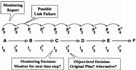
The sequence of object-level and monitoring decisions, and the points at which one's belief state will be updated, are il­ lustrated graphically in Figure 2 (other models of sequenc­ ing are possible however). At any point in time 1 :::; t :=:; n, assuming the agent is still able to execute the original plan rr, the agent makes two decisions in sequence. First it can request the monitoring of any action ak for any k 2: t. The observation reports obtained are used to update its cur­ rent belief state Pt to obtain a new distribution over pre­ conditions P/. Precondition independence means that this distribution can be factored into n distributions over indi­ vidual preconditions. Given this updated belief state, the agent now makes an object-level action choice: it can ei­ ther continue with the original plan rr and execute action a t , or it can abandon the plan and execute the alternative plan rr t . If the original plan is abandoned due to the pos­ sibility of link failure, then no future decisions need to be made: we assume that rr t can be executed without diffi­ culty to provide value v(rr t ). If a t is executed, any precon­ dition's status can change: the system dynamics determine the probability with which this occurs. The agent can up­ date its belief state from P/ to Pt + l reflecting the possible changes. As a consequence, there are two decision stages for each plan step: a monitoring stage with a decision at

6 More realistic models that distinguish the costs of continuing vs. intermittent monitoring could also be adopted.

timet, where one decides which preconditions to monitor; and an action stage decision at timet+, the decision regard­ ing which object-level action to execute (i.e., to continue or abandon the plan).

2.3 A POMDP Formulation

Optimal monitoring decisions can be determined by cast­ ing the problem as a POMDP and solving using standard dynamic programming methods [15, 11].

A POMDP can be viewed as a fully observable Markov decision process whose state space consists of probability distribution over underlying system states, or belief states. While the set of belief states is continuous (with dimension lSI -1), Sondik [15] showed that the k-stage-to-go value functions Vk of a finite-horizon POMDP is piecewise linear and convex (p.w.l.c.) and thus can be represented finitely using a collection of linear functions over belief space, or a-vectors. Specifically, given such a collection N k of lSI­ dimensional a-vectors, Vk(b) = max{b ·a: a E N k }.

The sequence of value functions Vk (or more accurately, their representation as sets N k ) can be computed by dy­ namic programming. We describe the basic intuitions using Monahan's [12] algorithm since it is conceptually straight­ forward. However, we tailor the presentation to our mon­ itoring problem. We assume an n-step plan monitoring problem with n action stages and n monitoring stages. The final decision occurs at time n+. A decision to continue with the last step of the original plan or to abandon the plan is made based on the belief state b n +. The value of aban­ doning the plan is v ( rr n ) regardless of the true state: hence the Q-function Q;b-;; n for action aban, where Q;b-;; n (b) is the value of aban at belief state b, can be represented by the con­ stant vector aaban with entries v( rr n)· The value of cont (i.e., attempting to continue the original plan) is simply v(rr) if the final precondition holds and v ( rr�) if it does not. Thus Q�otr ( b) = b · aconr. where acont is the vector with entries v ( rr) for each state where the precondition holds, and v ( rr�) where it doesn't. The value function v n + is thus repre­ sentable by N n + comprising these two vectors. It is clear that v n + is p.w.l.c. We note that each vector is associated with a specific action: if

then the optimal choice is cont, otherwise it is aban. More generally, as we see below, vectors denote the value of ex­ ecuting a complete course of action (or conditional plan) over the remainder of the problem horizon.

Given N t + for the tth action stage, we can compute N t for the preceding monitoring stage as follows. One can choose to monitor any subset of the remaining t preconditions.; thus a monitoring action refers to some collection of indi­ vidual monitoring actions. Any such compound monitoring action chosen involving k :::; t preconditions gives rise to 2k possible observations (2 observations for each observed condition). Since a different course of action can be pur­ sued after each distinct observation, we define the set ob­ servation strategies OS� for time t and monitoring action m to be the set of mappings u : Zm -+ N t + that associate

a subsequent a-vector with each possible observation (note that each vector has a conditional plan associated with it). The value of executing m together with u is again a linear function of the belief state. Specifically, for each state s the probability Pr(zls) of any observation z is fixed, and the Q-value of u at s is:

The Q-value of u can thus be represented by the vector a" with sth component Q( u, s); and Q t ( u, b) = b ·a" for any belief state b. The best monitoring action and observation strategy at belief state b is simply that which has maximum expected value at b; thus the value of optimal monitoring can be represented by the collection of a-vectors induced by the strategies in { OSm : m E M}. For each a-vector in this set we record the a p propriate monitoring action: if a" corresponds to u E OSm, we associate m with a". 7

Finally, given the value function � t + l for the t +1st moni­ toring stage, it is a simple matter to compute the value func­ tion � t + for the tth action stage. The decision at timet+ is, again, whether to continue the original plan 1r or abandon it (executing 1rt). If the agent persists with 1r for one addi­ tional step, value is given almost directly by v t + l : once the specific step of 1r is executed, the agent can act optimally by selecting the subsequent course of action dictated by v t + l . Each course of action corresponds to some a E � t + l . The value of continuing with 1r at a specific state s followed by implementing a is given by:

for any s where the precondition for a t holds. At all other s, Q t +(a, s) = v ( 1r { ) . The value of continuing with 1r can therefore be represented by:

With each such vector we associate the action cont. If 1r is abandoned, the value obtained is the constant c( 1rt) (inde­ pendent of the state s ). Thus

where the action aban is associated with the constant vector.

Apart from the division into action and monitoring stages, this algorithm is essentially that proposed by Monahan with one exception. The collections of a-vectors defined above typically contain many dominated vectors that do not max­ imize value at any belief state. Monahan's algorithm in­ volves an additional pruning phase where dominated vec­ tors are removed at each stage before moving to the next stage. This provides tremendous computational benefit.

7 We note that not monitoring any precondition corresponds to choosing the empty subset of conditions above. The Q-value of this action is simply identical to the value function vt+' thus the set l{ t + can be copied directly into l{ t .

Other algorithms, including linear support [5] and Witness [ 4] proceed by directly identifying only (or primarily) non­ dominated vectors and thus require little or no pruning, and tend to be more efficient still. Our results in Section 4 are all based on the Witness algorithm.

Given a collection of �-sets, implementation of the moni­ toring and execution policy requires that the agent maintain and update its belief state b over time. At each (monitoring or action) stage k, b is applied to each vector a E � k to de­ termine b · a, and the action associated with the maximiz­ ing vector is executed. Actions are either monitoring deci­ sions for the remaining preconditions, or "continue" deci­ sions. At action stages, the single aban-vector has constant value, so the cant-vectors need only be searched until one better than the sole aban-vector is found.

While this model is conceptually appealing, it is computa­ tionally intractable for all but the most trivial plan monitor­ ing problems. For plans involving n preconditions, there are 2n states, as many as 2n monitoring actions, and up to 2n observations. Present (exact) POMDP algorithms can at best deal with problems involving a thousand states and are highly sensitive to the number of actions and observations. The solution of the plan monitoring POMDP can be well beyond the reach of state-of-the-art algorithms like Witness for three step plans. Clearly, some problem decomposition and approximation is required if the decision-theoretic ap­ proach is to be practical.

3 Heuristic Monitoring

In this section we consider two alternative models for solv­ ing the monitoring problem that are vastly superior to the full POMDP formulation computationally. Intuitively, for a planning problem with n stages, we solve n independent monitoring problems, one for each precondition (recall that we assume a single precondition per action). The solutions to these individual problems are then combined online. In particular, at a given decision stage, whether action or mon­ itoring, we have access to the value functions and policy de­ cisions for the individual problems at that stage, as well as the current belief state. These are used to determine an ap­ propriate choice of action for the original monitoring prob­ lem at that point.

3.1 Solving Single-Failure POMDPs

For each precondition (or action) a t in ann-stage plan, we consider the problem of optimally monitoring a t over the interval [1, t] under the assumption that this is the only pre­ condition that can fail. This is a t-stage POMDP with ac­ tion and monitoring stages as above. The key difference is that decisions are based on belief in the state of that pre­ condition alone. As such the corresponding POMDP has only two states, one monitoring action, and two observa­ tions. This tth single-failure monitoring problem is there­ fore generally very easily solved. The solution of each of n single-failure problems provides us with at-stage value function for the tth problem, this value function consisting oft sets of a-vectors, �f, · · · , ��- Thus the value functions for all n problems can be represented in O(l · n2 ) space,

where l is a bound on the size of any N-set.

3.2 Naive Policy Combination

Assume that then single-failure monitoring POMDPs for an n-stage planning problem have been solved. At any given monitoring stage t, the individual policies for each action ak (t :S k :S n) will each require that their action either be monitored or not. At each action stage t+, the po­ lices for each ak will either suggest that the original plan be abandoned or continued.

Our Naive Policy Combination (NPC) algorithm works as follows. The agent maintains a factored belief state {b1, · · ·, bn ) over the n individual preconditions (since these are independent). At each monitoring stage t, the in­ dividual value functions NL (t :S k :S n) are applied to the bk, and the monitoring decision for each ak made on this ba­ sis. Thus the actual monitoring action m = (m t , · · · , mn) executed has mk assigned to "monitor" iff monitoring is op­ timal for the kth subproblem. At each action stage t+, the individual value functions Nt+ (t :S k :S n) are applied to the bk, and the object-level action decision for each ak determined. The action cant is executed if each of the indi­ vidual policies suggest continuing. The action aban is exe­ cuted if any of the individual policies suggest abandonment.

3.3 Value Function Adjustment

In the NPC strategy described above, if any monitoring problem requires that the plan be abandoned, then abandon­ ment is (globally) optimal. However, continuing may not necessarily be optimal. Consider for instance that each pre­ condition may be probable enough that the "abandonment threshold" for the individual problem is not reached. How­ ever, when the probability of failure as a whole is consid­ ered, abandonment may, in fact, be appropriate.

We can perform some simple adjustments to the individ­ ual value functions to attain a more accurate estimate of the value of continuing a plan. Consider the decision at action stage t+, with individual value functions Nt+ (t :S k :S n) and belief state bk (1 :S k :S n ). The value v�+ ( bn ) is an accurate reflection of value assuming that all preconditions a j (j < n) preceding an are OK. Specifically, the course of action associated with any o: E N;,+ does in fact have value bn · o:. The value v:� 1 ( b n -1) is also accurate under the as­ sumption that the preceding conditions a j (j < n1) are OK as well as condition an. However, if we wish to account for the fact that an may have failed, we can adjust the value function to reflect the fact that the impact of an failing is captured by the value v�+(bn) just calculated.

This adjustment can be effected by noting that for any o: E N�� 1 , its ith componento:; is given by pfv('rr) +(1-pi)x, where pf denotes the probability of successfully reaching and executing action an-1 under the conditional plan re­ flected by o: at state s;, and x is some indeterminate quan­ tity (reflecting average value of plan abandonment/failure). Once we execute an-I. however, the value v(1r) is not as­ sured for action an may fail, or be abandoned, etc. To ap­ proximate the influence of this possibility, we can replace v ( 1r ) in the above expression with the expected value of the nth monitoring problem, v�+ ( b n ); we replace each compo­ nent o:; of o: with

This value-adjusted estimate offers a better picture of the overall value of executing the conditional plan associated with o:, taking into account the influence of the later pre­ condition. We then take V�� 1 (bn-d to be computed w.r.t. the adjusted o:-vectors ��� 1 .

Our Value-Adjusted Policy Combination (VAPC) algorithm works as follows. Monitoring decisions are made precisely as in NPC. The action decision at stage t+ is made by work�t + ing backwards from stage n to stage t. We define N k for each t :S k < n to be the set of value-adjusted vectors using v:t1 (bk + d (i.e., each o: E Nt+ is replaced by its value-adjusted counterpart using v:tl (bk +l ) as the substi­ tute for v(7r)). v t + is in tum defined as the value function induced by the value-adjusted N-set �L "t 1 . This recursion is grounded at stage n where �;,+ = N;,+. Algorithmi­ cally, this process can be implemented efficiently. Starting at stage n, the continue/abandon decision is made for an. If the decision is aban, a global abandon decision is made and we terminate. Otherwise, we move to stage n1, comput­ ing the adjusted set ��� 1 using v�+(bn) (note that v�+(bn) is computed as a by-productof the decision for an). A deci­ sion to continue or abandon is then computed for an-1 us­ ing ��� 1 . If aban is chosen, again we abandon the plan, otherwise we move to stage n -2, adjusting its o:-vectors using the (already-computed) value V��1 (bn-d· This is re­ peated back to at , terminating whenever one action calls for abandonment, or when at is reached with all actions calling for continuation.

The probabilities pf can can be computed easily during the dynamic programming solution of the individual monitor­ ing problem for ak. For each o:-vector ( v1, v 2 ) at any stage, we compute a corresponding probability vector (P?, P2). (there are two states, one denoting ak 's precondition OK, and one its failure). At stage n, these probabilities are ei­ ther 0 or 1 (recall they are a function of the state, not belief state). At any earlier stage, they are calculated as a function of the probabilities associated with the following stage, in exactly the same way that the values v; for the o:-vector are computed. This adds minimal computation time to dynamic programming and requires only that we store an extra col­ lection of vectors: a probability vector for every o:-vector.

The additional online adjustment phase ofVAPC makes on­ line policy combination slightly more complex than NPC: VAPC requires roughly twice the time to come to a deci­ sion at any stage. Both, however, are linear in the sum of the sizes of the value functions being used. If the vector sets for each subproblem are bounded in size, then this is linear in the plan size (number of stages). Thus both methods are efficient in their online computations.

4 Empirical Results

In this section we describe empirical results suggesting that the computation time required to solve monitoring prob­ lems using our approximation technique is negligible when compared to the full POMDP model, and that it scales very well to plans involving many hundreds of steps. We also provide evidence that the solution qu:!lity is generally quite good. Our ability to do so is limited however by the fact that computing optimal solutions for all but the most triv­ ial problems is a practical impossibility. The Witness algo­ rithm is used to solve all POMDPs (both the full POMDP and the single-failure POMDPs for each problem).8

We begin with a simple three-stage problem. This problem has characteristics that make it relatively "easy" to solve: precondition failure has small probability and no precon­ dition can become OK once it has failed. The failure and abandonment costs do not impose severe penalties, so the value function has few components.9 This full POMDP was still very difficult to solve, requiring 9608 seconds (2.7 hrs) of CPU time for Witness. Despite this the largest value function (at the first monitoring stage) had only eight vec­ tors (each precondition was monitored in some of the cor­ responding actions, though not every combined monitoring action was part of the optimal policy). In contrast, the ap­ proximation algorithm produced the collection of compo­ nent value functions in 5.78 seconds (5.86 seconds if ad­ justment probabilities are computed, 2. 71 seconds if Mona­ han's algorithm is used rather than Witness). 1 0 The largest �-set had only 4 vectors.

On other three-stage problems, we were unable to get Wit­ ness to run to completion in a reasonable time on the full POMDP. For instance, in one example with a more com­ plex value function, Witness was terminated after 76035 seconds (over 21 hours of CPU time) with an agenda (see [4] for details) of over 10000 vectors (with indications that the agenda was still growing). In contrast, the approxima­ tion method required only 5.06 seconds (5.08 if adjustment probabilities are computed). 11

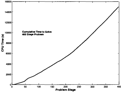
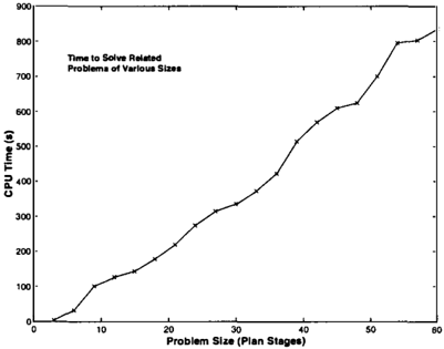
The scaling of the approximation algorithms is illustrated in Figure 3, where solution time is plotted as a function of problem size for a series of related problems. In this se­ quence, the scaling appears to be nearly linear, though in fact this is largely due to the fact that the value functions tend to simplify as the horizon grows. In general, we expect

8 Algorithms are implemented in Matlab and run under Linux on a 550MHz Pill architecture with 512Mb of memory.

9 Specifically, each of the tltree preconditions had a 0.01 chance of failing at each stage, and observation of each precondition has a 0.1 false negative rate and a 0.3 false positive rate. Successful plan value is 20; alternative plans have value 12, 8 and 4, respectively, at steps 1 through 3; plan failure values are 10, 5, and 2 (hence plan failure does not impose great cost); observation costs are 0.5, 0.5 and 0. 7 for preconditions I through 3, respectively.

11 This problem is similar to the one above but with a higher precondition failure rate of 0.05, more accurate observations (0.2 false positive rate), smaller observation costs (0.3), and greater cost due to plan failure (i.e., greater difference between success­ ful and failed plan values).

10 Monahan's algoritltms tends to work better than Witness if the value functions are very compact.

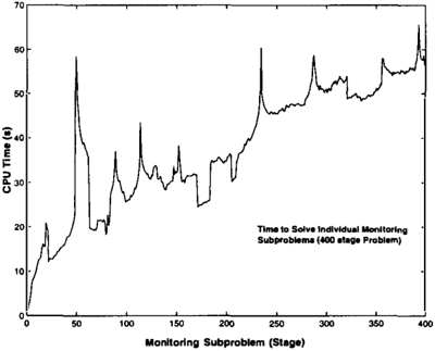
scaling to be quadratic in problem size. The (rather slow) quadratic growth is evident in Figures 4 and 5, where the solution times for the component single-failure monitoring problems in a 400-step plan are shown, as well as the cumu­ lative solution time (thus this 400-step monitoring problem is solved in about 4 hours). 1 2

The efficiency gains of this approach cost very little in terms of solution quality. We compare solution quality of our approximations to the optimal solution for the three­ stage problem we were able to solve optimally (see details above). This comparison is made by comparing the ex­ pected value of the policy induced by NPC and V APC with the optimal value, at a number of different belief states. We sampled 1331 belief states uniformly distributed over belief space: for each of the three variables, each degree of belief between 0 and 1 was sampled at intervals of 0 .1. Over these 1331 states, the average relative error in decision quality for NPC was 0.049, and for VAPC, 0.047; thus on average both strategies give rise to policies whose value is within 5% of optimal. The maximum relative error at any belief state is

12 Note tltat tlte full POMDP has 2 400 states, 2 400 monitoring actions and up to 2 400 observations for certain monitoring actions.

J

0.166 for NPC and 0.142 for VAPC. The sacrifice in deci­ sion quality seems a small price to pay for the vast differ­ ence in computational effort.

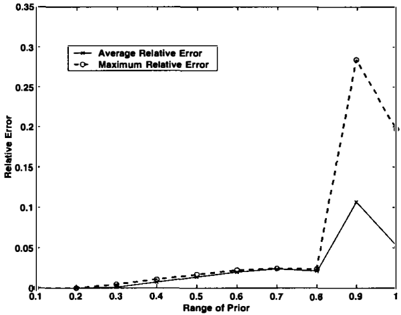
More interesting is the fact that the decision quality tends to vary significantly in different parts of belief space. We plot the relative value error for "high prior" belief states in Fig­ ure 6 (here we only show NPC). At each pointp (e.g., 0.7), we show the relative errors over all sampled belief states where each precondition is restricted to have prior proba­ bility between p and 1 in increments of 0.1 (e.g., at 0.7 we see the error ranging over belief states, for each variable, in the set {0.7, 0.8, 0.9, 1.0} ). We see here that the relative e ?" or for our approximation technique tends to decrease sig­ mficantly at belief states with high prior precondition prob­ ability. At .9 and above, all decisions are in fact optimal. At .8 and above, average error is about 0.1 per cent. This is important because plans involving such preconditions are likely to be invoked only when the preconditions are rea­ sonably likely to hold.

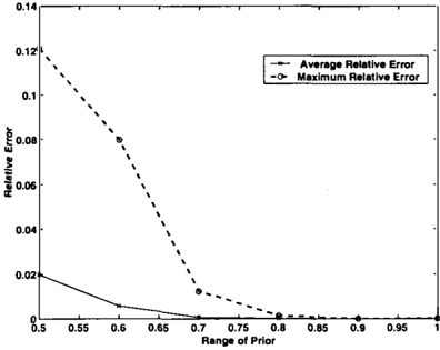
A similar plot for "low prior" states is shown in Figure 7, where relative error for belief states ranging from p down to 0 (again in 0.1 increments) is plotted. Again we note that the error tends to be most pronounced in the intermediate

belief states.

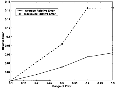
Finally, we compare the relative value attained by NPC and VAPC on a slightly larger 5-stage problem. 1 3 The solu­ tionof this problem requires 16.04 seconds (16.09when ad­ justment probabilities are computed). Figure 8 illustrates the relative improvement of VAPC over NPC on a num­ ber of belief state ranges. Each point p shows the aver­ age and maximum relative improvement of V APC over the 243 belief states where each of the 5 variables has proba­ bility in {p 0.1, p 0.05, p}. In this problem, the in­ dividual value functions tend to be reasonably sensitive in the choice of whether to continue of abandon in the neigh­ borhood [0.8, 0.9]. VAPC offers considerable advantage of NPC areas around this point, with average improvement in decision quality of nearly 11% in this range and maximum improvement of 28.5%.

1 3 Problem parameters: 0.05 probability of precondition failure and 0.1 chance of precondition repair; observations have a 0.1 false negati y e and a 0. 2 false positive rate; successful plan value is 40; altemauve plan values are 25, 18, 12, 7, and 6; failure values are 12, 11, 7, 5, and 2; observation costs range from 0.3 to 0.5.

5 Concluding Remarks

We have described a decision-theoretic model for optimal plan monitoring that takes into account monitoring costs, the probability of precondition failure, and the value of al­ ternative plans. While this model is conceptually appeal­ ing, it is wildly intractable, leading us to develop approxi­ mation methods that scale very well with plan size and seem to make small sacrifices in decision quality. This approach makes decision-theoretic monitoring practical for complex planning and monitoring problems.

There are a number of simple improvements that can be made to this approach. One involves scaling to large plan­ ning problems through the use of critical points. One can identify a subset of a plan's actions to monitor-rather than monitoring all n actions-by considering the difference in the value of the alternative plans 7ft at various points. If v ( 7rt) is not much less than v ( 7r t +d it may be reasonable to simply ignore action at in one's monitoring problem. By judicious selection of such critical points (i.e., points in the plan such that the cost of abandoning the plan once commit­ ting to them is very high), the number of stages and precon­ ditions one needs in a monitoring problem can be reduced.

The extension of this model to handle correlated precon­ dition failures is critical for many applications. Dealing with correlations should prove to be fairly easy, using, say, Bayesian networks to represent existing independence in the transition model and the belief state. The same basic ap­ proach to decomposing the POMDP into individual moni­ toring problems is still applicable, though the value adjust­ ment phase in the VAPC technique will require modifica­ tion. Other directions for future research include develop­ ing formal error bounds for this approach, the incorpora­ tion of more sophisticated cost and value models for the un­ derlying planning domain, and extending the model to deal with partially-ordered plans.

Acknowledgements Many thanks to Pascal Poupart and Manuela Veloso for their helpful discussion, as well as to the reviewers for their comments. This research was sup­ ported by IRIS Phase 3 Project BAC, NSERC Research Grant OGP0121843, and the DARPA Co-ABS program (through Stanford University contract F30602-98-C-0214).

References

1. K. J. Astrom. Optimal control of Markov decision processes with incomplete state estimation. J. Math. Anal. Appl., 10:174-205, 1965.
2. Ella M. Atkins, Edmund H. Durfee, and Kang G. Shin. Detecting and reacting to unplanned-for world states. In Proceedings of the Fourteenth National Conference on Artificial Intelligence, pages 571-576, Providence, RI, 1997.
3. Craig Boutilier, Richard Dearden, and Moises Gold­ szmidt. Exploiting structure in policy construction. In Proceedings of the Fourteenth International Joint Conference on Artificial Intelligence, pages 11041111, Montreal, 1995.
4. Anthony R. Cassandra, Leslie Pack Kaelbling, and Michael L. Littman. Acting optimally in partially observable stochastic domains. In Proceedings of the Twelfth National Conference on Artificial Intelli­ gence, pages 1023-1028, Seattle, 1994.
5. Hsien-Te Cheng. Algorithms for Partially Observable Markov Decision Processes. PhD thesis, University of British Columbia, Vancouver, 1988.
6. Thomas Dean and Keiji Kanazawa. A model for rea­ soning about persistence and causation. Computa­ tional Intelligence, 5(3): 142-150, 1989.
7. Joaquin L. Fernandez and Reid Simmons. Robust ex­ ecution monitoring for navigation plans. In Interna­ tional Conference on Intelligent Robotic Systems, Vic­ toria, BC, 1998.
8. R. James Firby. Adaptive Execution in Complex Dy­ namic Worlds. PhD thesis, Yale University, New Haven, 1989.
9. Steve Hanks and Drew V. McDermott. Modeling a dynamic and uncertain world i: Symbolic and proba­ bilistic reasoning about change. Artificial Intelligence, 1994.
10. Nicholas Kushmerick, Steve Hanks, and Daniel Weld. An algorithm for probabilistic least­ commitment planning. In Proceedings of the Twelfth National Conference on Artificial Intelligence, pages 1073-1078, Seattle, 1994.
11. William S. Lovejoy. A survey of algorithmic methods for partially observed Markov decision processes. An­ nals of Operations Research, 28:47-66, 1991.
12. [ 12] George E. Monahan. A survey of partially observable Markov decision processes: Theory, models and algo­ rithms. Management Science, 28:1-16, 1982.
13. [ 13] Louise Pryor and Gregg Collins. Planning for contin­ gencies: A decision-based approach. Journal of Arti­ ficial Intelligence Research, pages 287-339, 1996.
14. M. J. Schoppers. Universal plans for reactive robots in unpredictable environments. In Proceedings of the Tenth International Joint Conference on Artificial In­ telligence, pages 1039-1046, Milan, 1987.
15. Richard D. Smallwood and Edward J. Sondik. The optimal control of partially observable Markov pro­ cesses over a finite horizon. Operations Research, 21:1071-1088, 1973.
16. Manuela M. Veloso, Martha E. Pollack, and Michael T. Cox. Rationale-based monitoring for con­ tinuous planning in dynamic environments. In Pro­ ceedings of the Fourth International Conference on AI Planning Systems, pages 171-179, Pittsburgh, 1998.