Approximations for Decision Making in the Dempster-Shafer Theory of Evidence

Mathias Bauer

German Research Center for Artificial Intelligence (DFKI) Stuhlsatzenhausweg 3

66123 Saarbriicken, GERMANY

email: [email protected]

Abstract

The computational complexity of reasoning within the Dempster-Shafer theory of evidence is one of the main points of criticism this formalism has to face. To overcome this difficulty various approximation algorithms have been suggested that aim at reducing the number of focal elements in the belief functions involved. Besides intro­ ducing a new algorithm using this method, this paper describes an empirical study that examines the appropriateness of these approximation pro­ cedures in decision making situations. It presents the empirical findings and discusses the various tradeoffs that have to be taken into account when actually applying one of these methods.

1 Introduction

The complexity of the computations that have to be car­ ried out in the Dempster-Shafer theory of evidence (DST) [Dempster, 1967; Shafer, 1976] is one of the main points of criticism this formalism has to face. In fact, [Orponen, 1990] shows that the combination of two basic probability assignments (bpa' s) using Dempster's rule is #P-complete. 1 To overcome this difficulty various approximation methods have been suggested. While some of them concentrate on the processing of particular types of information only­ e.g. the methods proposed in [Barnett, 1981] and [Gordon & Shortliffe, 1985]--others try to attack this problem for arbitrary bodies of evidence.

The number of focal elements in the belief functions under consideration heavily influences the computational com­ plexity of combining various independent pieces of evi­ dence. As a consequence, [Voorbraak, 1989], [Tessem, I993], and [Lowrance, Garvey, & Strat, 1986] suggest ap­ proximations that aim at reducing this influence factor by removing focal elements and/or redistributing the corre­ sponding numerical values.

An empirical study presented in [Tessem, I993] investigates

1The class #P is a functional analogue of the class NP of decision problems.

the quality of the approximations so obtained by considering the average maximal deviation from function values that are relevant to decision making. A second criterion to assess the quality of an approximation is its ability to induce some "structure" on the given information, thus allowing an adequate presentation of the essentials of its contents to a user.

While this study focused on the quantitative aspects of de­ cision making only, the quality of a decision is more impor­ tant in many applications. That is, whenever the numbers only serve as a means for finding the best candidate among a number of alternatives, the numerical deviation from the ac­ tual values is of secondary interest only. As a consequence the empirical study presented in this paper will consider both numerical and qualitative aspects when evaluating the appropriateness of various approximation algorithms for ef­ ficient decision making. Building upon the methodology described in [Tessem, 1993] new measures capturing the deviation from an optimal choice are introduced and the actual output size of the methods under consideration is recorded, thus providing the basis for discussing the vari­ ous tradeoffs associated with the application of one of the algorithms presented.

In addition to investigating the properties of various al­ gorithms known from the literature, this paper also intro­ duces a new approximation method-the D I algorithm­ and compares its performance with that of the other candi­ dates.

The rest of this paper is organized as follows. Section 2 reviews the basic notions of DST and motivates the need for approximate computations. Section 3 discusses four approximation procedures including the new D I algorithm before Section 4 describes the testbed used and interprets the empirical results. Finally, Section 5 concludes with a brief summary and a reference to related work. An appendix contains the graphs illustrating the empirical findings.

2 The Need for Approximations

The basic carrier of information in the Dempster-Shafer theory of evidence (DST) is a basic probability assignment

(bpa),2 a function m : 2 e --+ [0, I] that assigns a numerical value to each subset of a given frame of discernment 8 and satisfies the properties

• m(0) = Oand
• I:A<;e m(A) = 1.

Subsets A � 8 with m(A) > 0 are called the focal ele­ ments of m. Two bpa' s mi and m2 can be combined using Dempster's rule [Dempster, 1967):

Dealing with bpa' s brings about both representational and computational complexity problems that are discussed in [Orponen, 1990) where the combination of various pieces of evidence using Dempster's rule is shown to be #P-complete. Given a frame of discernment of size 181 = N, a bpa m can have up to 2 N focal elements all of which have to be represented explicitly to capture the complete information encoded in m. Furthermore, the combination of two bpa' s requires computation of up to 2 N +I intersections.

Reducing the number of focal elements of the bpa' s under consideration while retaining the essence of the informa­ tion they represent is thus a viable way to overcome these problems. The next section will present a number of ap­ proximation algorithms all of which make use of this basic idea.

3 Approximation Algorithms

This section reviews various approximation algorithms known from the literature, introduces the new D 1 algo­ rithm, and discusses their basic characteristics including their respective computational complexity and the size of their output in terms of the number of focal elements left after approximation. Combined with the empirical results described in Section 4.2, this will form the basis for the evaluation of the various tradeoffs associated with the ap­ plication of a particular approximation method in decision making situations .

3.1 The Bayesian Approximation

The Bayesian approximation [Voorbraak, 1989) reduces a given bpa m to a (discrete) probability distribution, i.e. only singleton subsets of the frame of discernment are allowed to be focal elements of the approximated version m of m:

20r equivalently one of the uniquel y derivable belief or plau­ sibilit y functions.

As a consequence m can have at most 181 focal elements. Given a bpa m with n focal elements, its Bayesian approx­ imation can be computed in time O(n ·181).

Remarks:

1. mi E9 m2 = m1 E9 m2, i.e. the order of combination and approximation does not influence the final result. Among all the algorithms taken into consideration in this paper, the Bayesian approximation is the only one with this property.
2. If mi is a Bayesian bpa (i.e. mi has only singleton focal elements), then mi $ m2 = m1 E9 m2.

The following example will be used throughout the rest of this section to illustrate the effects of the various approxi­ mation methods described.

Example:

Let m be a bpa over the frame of discernment 8 {a, b, c, d, e} with the values

Applying the Bayesian approximation to m yields the fol­ lowing result

This example demonstrates that the application of this ap­ proximation method is not reasonable in cases where the number of focal elements of the input bpa m itself is:::; 101.

3.2 The k-1-x Method

The basic idea of this approximation introduced in [Tessem, 1993] is to incorporate only the highest valued focal ele­ ments of the original bpa into the approximation mktx as long as at least k and at most l focal elements remain and the sum of them-values of the remaining focal elements is at least I -x where x E [0, 1 [. Finally the remaining values are normalized in order to guarantee the basic properties of a bpa (see Section 2). The exact definition of this algorithm is given in Figure 1. For a bpa m with n focal elements the approximation mktx can be computed in time O(n ·log n).

Example:

For the bpa mas given in (1) and the values k = 2, l = 3,

begin k-1-x-approximation(m, k, l, x)

sort the subsets of e w.r.t. their m-values total mass := 0 %total mass of m�o1x so far

while m contains focal elements and

% number of focal elements of m�o1:z:

(f::;

l)

and or

((f < do add next focal element A of m to m�ozx k)

(totalmass

totalmass := totalmass + m(A)

od normalize the values of m�ozx

end and x = 0.1, the following results are obtained.

Removing { c, d} and { d, e }-each with a value of 0.05from m was sufficient to satisfy both the constraints con­ cerning the number of focal elements left and the numerical mass deleted. In this case, normalizing the remaining val­ ues is equivalent to dividing them by 0.9-the value of 1(m({c,d}) + m({d,e})).

3.3 Summarization

Similar to the k-l-x procedure, the summarization method [Lowrance, Garvey, & Strat, 1986] leaves the best-valued focal elements of the bpa under consideration unchanged. The numerical values of the remaining focal elements are accumulated and assigned to the set-theoretic union of the corresponding subsets of e.

Let k be the number of focal elements to be contained in the approximation ms o f a given b p a m. M denotes the set of the k 1 subsets of 0 with the highest values in m. Then ms is given by

where Ao is uniquely determined by

The summarization of a bpa with n focal elements can be computed in time O(n).

< l- x))

Example:

For the b p a m from (1) and k == 3, ms has the following values.

In this case Ao corresponds to { c, d, e}, the set M of the k I best-valued focal elements of m contains {a, b} and {a, c, d}.

3.4 The Dl Approximation

Let m be a bpa to be approximated. Again k is the desired number of focal elements of the approximated bpa mD. Furthermore, let M+ denote the set of the k 1 focal ele­ ments of m with the highest values, Mthe set containing all other focal elements of m:

The crucial idea of the Dl algorithm is to keep all the members of M+ as focal elements of mD and to distribute the numerical values of the elements in Mamong them. This distribution works as follows. Given a focal element A E Mof m, the collection MA of supersets of A in M+ is computed. The value m(A) is dispensed uniformly among the (set-theoretically) smallest members of MA.

In case MA is empty, i.e. M+ contains no superset of A, the set MA. is constructed:

Again m(A) is shared among the smallest members of MA.. The exact value to be assigned to a focal element depends on the size of its intersection with A. This procedure is invoked recursively until all of m(A) could be assigned to the members of M+ or the set MA becomes empty. In this case the remaining value is assigned to 0 which thus becomes a focal element of mD. The DI algorithm is described in detail in Figure 2.

The approximation of a bpa with n focal elements can be computed in time O(k · (n- k)).

Remarks:

1. This approximation method is conservative in that the numerical values of focal elements to be removed are exclusively assigned to (set-theoretically) larger sub­ sets of 0, i.e. the approximated version ffiD represents information that is less specific than the one originally encoded in m.
2. The distribution of the value m(A) of a focal element A E Mamong its supersets is intended to bring about minimal deviations in the pignistic probability induced by mD (see Section 4). This effect is even increased

begin DLapproximation(m, M+, M-) forall A EM+ end do mD(A) := m ( A ) od mD(E>) := m(E>) forall A EMdo distribute( A, m(A), IAI) od procedure distribute( A: set, val: real, limit: in t eger ) MA :={BE M+ I A c B} if MA -I- 0 then % case 1: M+ contains supersets of A MA := {B E MA liB I minimal in M A } forall BEMA do %uniform distribution ofm(A) among the members of M A: mD(B) := mD(B) + (1/IMAI) ·val od else % case 2: M+ contains no supersets of A fi MA_ := {B E M+ IIBI ::2:: limit, An B -I- 0} if MA_ = 0 then mD(E>) := mD(E>) +val else hlp:= 0 %part of m ( A ) already distributed fi MA := { BE MA. I I B I minimal in MA_} %let MA = {B,, ... , B1} % detennine portion of elements of A occurring in the various B;: t . · -I u�=' B; n AI raw.I AI %compute total number of "shares": n u m b e r := z::::=l IB; n AI forall BEMA do share := (IBn AI/ number)· ratio· val mv(B) := mv(B) +share hlp := hlp + share od if ratio< l then Arest :=A\ ul=1B; %remainder of A if Arest -:f. 0 fi then distribute(Arest, valhlp, limit) fi

by the concentration on the smallest possible supersets of A.

Example:

The D1 algorithm yields the following results for the bpa m from (1) and k = 3.

Obviously, {c}, {c,d}, and {d,e} belong toM-. The focal element {a, b} has an empty intersection with all of these sets. As a consequence its value remains unchanged. {a, c, d} is the only superset of { c} and { c, d} in M+, such that its value is increased by 0.10 + 0.05. Furthermore it covers half of the elements of { d, e} which adds up another 0.05/2 to the mD value of {a, c, d}. The rest is assigned to 9= {a,b,c,d,e}.

4 Empirical Tests and Results

A number of empirical tests were performed with the aim to investigate the appropriateness of the various approximation algorithms presented in the last section in decision making situations. Section 4.1 will describe the test environment and the error measures used to quantify the induced devia­ tions from an optimal decision, before Section 4.2 gives an overview of the results and discusses the tradeoffs associ­ ated with the application of a particular algorithm.

4.1 The Testbed

To arrive at comparable results, many parameters of the testbed were taken from [Tessem, 1993]. A frame of dis­ cernment of size 101 = 32 was assumed as the basis for all the tests. For each algorithm random bpa' s with 8 focal elements were generated and 5 combinations using Demp­ ster's rule were computed. 3 This was repeated more than 1000 times for each candidate. After each combination the results were approximated and evaluated w.r.t. the error measures described below.

Bpa' s are generated using exponentially distributed random numbers X and Y (with identical distributions) and the following algorithm:

rest:= I fori:= 1 to 7 do generate random number X randomly generate A � 8 m(A) := P(Y :s; X) · rest rest:= rest- m(A) od generate "new" A � e m(A) :=rest

3 [Tessem, 1993] also investigates bpa's with 2 and 4 focal elements.

Table 1: Quantitative Comparison of the Approximation Algorithms.

	average		minimum		maximum
	orig	approx	orig	approx	orig	approx
DL8	1624	7.90	213	7	7058	8
DL30	1616	29.93	208	29	4590	30
Summ_8	1680	8.00	209	8	5859	8
Summ30	1589	30.00	188	30	4404	30
Bayes	1632	29.32	217	23	5806	31
klx_01	1616	440.02	234	3	4447	1849
klx_30	1448	28.63	179	13	2763	30

This way a uniform distribution of numerical values among the focal elements is avoided, i.e. the random bpa' s are closer to "realistic" data where the information given sup­ ports the various alternatives to different degrees.

For the experiments the following parameter values were chosen. For Dl and the summarization algorithm the instantiations with k = 8 and k = 30----denoted by DL8, DL30, Summ_8, and Summ30, resp.-were con­ sidered. For the k-l-x method the parameter sets were k = 1,1 = oo,x = 0.014 and k = 1,1 = 3 0 , x = 1.0. The corresponding instantiations of this algorithm are de­ noted by klx_01 and klx30, resp. Recall that the Bayesian approximation algorithm is not parameterized.

All the error measures used are based on the pignistic prob­ ability Po induced by a bpa that can be considered the stan­ dard function for decision making in DST [Smets, 1988]. It is characterized by

To keep the results comparable to those obtained in [Tessem, 1993], the first error measure is identical to the one used there. It quantifies the maximal deviation in the pignistic probability induced by an approximated bpa. Let Po be the pignistic probability induced by the original version of a bpa m, Pa pp the one induced by its approximation m' (no matter which algorithm was applied). Then the error measure is defined as

This measure, however, does not reflect the quality of a decision based on Pap p . To do so, additional error measures are introduced. Let Xo, X a pp E e be characterized by the following properties:

4 The same values as in [Tessem, 1993].

i.e. x0 (xapp) is the best choice among all alternatives from e given Po cParr). In this situation, the quantities count the numbers of alternatives with a higher Papp value than x0 and a higher Po value than Xapp· resp. This means they reflect the rankings of x0 (the choice that should be made) on the basis of Papp and of Xapp (the choice actually made) on the basis of Po.

For example, given the concrete values of Error2(m') = 1 and Error3(m') = 2 for some approximated bpa m' means that the third best choice is made while the actual optimum is considered the second best alternative only.

Error3 is particularly important for the assessment of an approximation method w.r.t. decision making as it directly represents the quality of decision Xapp· A value of 0 indi­ cates that the approximation yields the same optimal choice as the original information. Note that in this case Error2 also assumes the value 0.

4.2 The Results

For a fair comparison of the various approximation algo­ rithms including a characterization of the respective trade­ offs associated with their application, it is not sufficient to merely consider these error measures. In addition the size of their output has to be taken into account to estimate the gain in runtime. Table 1 summarizes the average, mini­ mum, and maximum number of focal elements both in the original data and their approximations for each candidate algorithm after the fifth combination.

Remarks:

1. For technical reasons the algorithms were not run with identical test data. However, the statistical data in

Table l indicate that the average problem size was approximately equal for aJI candidates.

1. The extreme number of 1849 focal elements was pro­ duced by klx_Ol when the original bpa contained 3843 focal elements. The approximations generated by this algorithm exceeded 1000 focal elements in more than 7% of all cases.

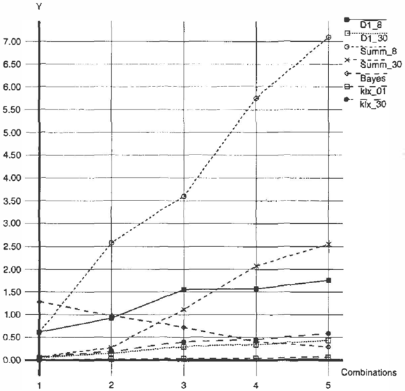
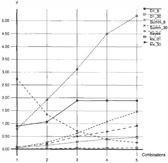
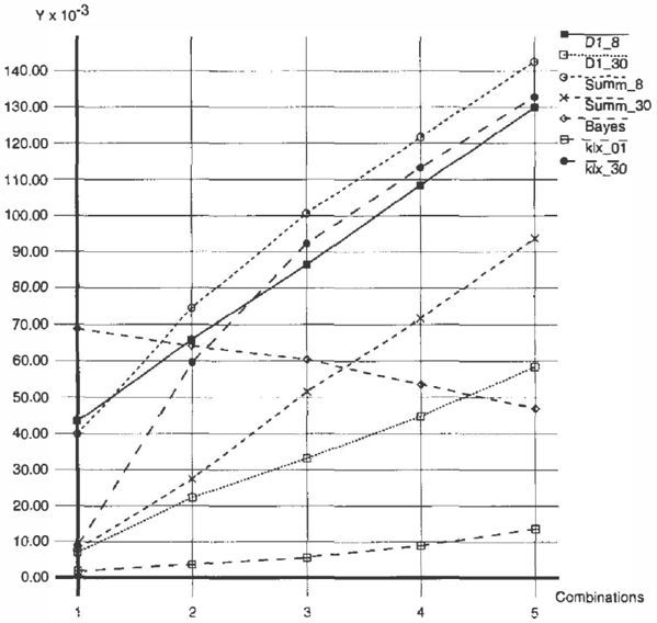
The Figures 3, 4, and 5 at the end of this paper (see Ap­ pendix A) depict the averaged results for the error measures described above.

In all three cases klx_01 reaches the best values. This is due to the fact that only relatively few focal elements with extremely low values are removed from the input data. The average size of a bpa approximated with this method is 440 focal elements, the maximum is even more than 1800 (see Table l ). As a consequence the gain in runtime is the least among all candidates-taking into account both the time to compute the combinations and the approximation itself. Restricting the number of focal elements as in klx30 improves this aspect but induces significant deviations in Error).

Compared to algorithms with similar output size, both ' in­ s t an tia t ion s of the summarization yield the worst values for all error measures.

The Bayesian approximation is the only one with improv­ ing values after several combinations. In [Tessem, 1993] this is explained by the fact that the result of combining several bpa' s becomes more and more specific and thus ap­ proximates a probability distribution. As a consequence this algorithm yields its worst results whenever decisions have to be made on the basis of little evidence only. After 4 to 5 combinations it reaches the level ofD130.

The errors induced by D 1 are relatively small even for the instantiation with 8 focal elements only (this is particu­ larly true for Error2 and Error3). This facilitates decision making in extremely time critical applications. The D l 30 instantiation yields the best values of all candidates (with the exception of klx_Ol) during the first combinations. Af­ ter the 4th to 5th step the Bayesian approximation starts to produce slightly better values.

What are the consequences for the selection of a particular algorithm in a given application? If t h e runtime behavior is not too critical, klx_Ol or similar instantiations of the k-1-x algorithm are the best choice.5 If only up to 181 focal elements are acceptable, Dl 30 and the Bayesian approxi­ mation yield the best results. The former is advantageous during the first combinations, while the latter is preferable during longer cycles. If time restrictions allow only very coarse approximations, D1 outperforms the competitors as the example of D 1_8 shows.

Remark: The positive results for the Bayesian approxima­ tion do not come for free. It c o l l ap ses the belief intervals [Bel(.), Pl(.)J into point values. As a consequence, the

5Further experiments showed that all 3 error measures grow approximately linearly with the value of x.

ability of DST to explicitly represent and deal with partial ignorance is lost.

5 Conclusion

The results presented in the preceding section clearly show that the "best" approximation algorithm with respect to de­ cision making does not exist. Instead the tradeoffs between the number of focal elem ent s remaining, the complexity of computing the approximation itself, and the quality of the decisions made have to be taken into account. However, it can be stated that the k-l-x algorithm, D l, and the Bayesian approximation yield definitely better results than the sum­ marization does. Given a particular application, a ranking of these three alternatives can be established on the basis of the discussion in Section 4.2.

This also applies to the consonant approximation [Dubois & Prade, 1990]. The test results of this approximation method were significantly worse than those of all other algorithms examined (as was already observed in [Tessem, 1993]). As a consequence this candidate was not further discussed in this paper.

In addition to the approximation methods presented here, several Monte-Carlo algorithms were suggested to make reasoning in the DST computationally feasible (e.g. [Wil­ son, 1991; Kreinovich et al., 1994]). Their application involves making a number of random choices on the ba­ sis of some probability distribution. Trying to arrive at a correct result with a certain probability, their usage can be motivated by the common observation that even the initial input data given by an expert are reliable only to a certain degree such that it is justifiable to have an algorithm the output of which is slightly incorrect in a limited number of cases [Kreinovich et al., 1994]. Future work will in­ clude the examination of the properties of such algorithms in practical applications.

Acknowledgements

This work was supported by the BMBF under grant ITW 9404 0 as part of the RAP project.

I'd like to thank my colleagues Dietmar Dengler and Harald Feibel for their comments on earlier versions of this paper and Patrick Brandmeier for his support in implementing the testbed and running the experiments.

A The Error Graphs

This appendix contains the graphs depicting the average values of the measures Error! through Error3 defined in Section 4.1 for each of the approximation methods dis­ cussed in Section 3 and the corresponding instantiations of their parameters mentioned above.

Figure 3: Results for Errorl.

2

3

4

Figure 4: Results for Error2.

5

References

• [ Barnett, 1981] Barnett, J. 1981. Computational Methods for a Mathematical Theory of Evidence. In Proceedings of the 7th International Joint Conference on Artificial Intelligence, 868-875.
• [ Dempster, 1967] Dempster, A. 1967. Upper and lower probabilities induced by a multivalued mapping. Annals of Mathematical Statistics 38:325-339.
• [ Dubois & Prade, 1990] Dubois, D., and Prade, H. 1990. Consonant approximations of belief functions. Interna­ tional Journal of Approximate Reasoning 4:419-449.
• [ Gordon & Shortliffe, 1985] Gordon, J., and Shortliffe, E. 1985. A Method for Managing Evidential Reasoning in a Hierarchical Hypothesis Space. Artificial Intelligence 26:323-357.
• [ Kreinovich et al., 1994] Kreinovich, V. Y.; Bernat, A.; Borrett, W; Mariscal, Y.; and Villa, E. 1994. Monte­ Carlo methods make Dempster-Shafer formalism feasi­ ble. In Yager, R. R.; Kacprzyk, J.; and Fedrizzi, M., eds., Advances in the Dempster-Shafer Theory of Evi­ dence. New York: Wiley. 175-191.
• [Lowrance, Garvey, & Strat, 1986] Lowrance, J.; Garvey, T.; and Strat, T. 1986. A Framework for Evidential­ Reasoning Systems. In Proceedings of the 5th National Conference of the American Association for Artificial Intelligence, 896-903.

.

• [ Orponen, 1990] Orponen, P. 1990. Dempster's Rule of Combination is # P-complete. Artificial Intelligence 44:245-253.
• [ Shafer, 1976] Shafer, G. 1976. A Mathematical Theory of Evidence. Princeton, NJ: Princeton University Press.
• [ Smets, 1988] Smets, P. 1988. Belief Functions versus Probability Functions. In Bouchon, B.; Saitta, L.; and Yager, R., eds., Uncertainty and Intelligent Systems, vol­ ume 313 of Lecture Notes in Computer Science, 17-24.
• [ Tessem, 1993] Tessem, B. 1993. Approximations for ef­ ficient computation in the theory of evidence. Artificial Intelligence 61:315-329.
• [ Voorbraak, 1989] Voorbraak,F. 1989. A Computationally Efficient Approximation ofDempster-Shafer Theory. In­ ternational Journal of Man-Machine Studies 30:525536.
• [Wilson, 1991] Wilson, N. 1991. A Monte-Carlo Algo­ rithm for Dempster-Shafer Belief. In D'Ambrosio, B.; Smets, P.; and Bonissone, P., eds., Proceedings of the Seventh Conference on Uncertainty in Artificial Intelli­ gence, 414-417.

5