Contents
1301.6692
Assessing the value of a candidate
Comparing belief function and possibility theories
Didier Dubois
Institut de Recherche en Informatique de Toulouse Universite Paul Sabatier, 118 route de Narbonne 31062 Toulouse Cedex 4, France
Michel Grabisch Thomson-CSF, Corporate Research Laboratory Domaine de Corbeville 91404 Orsay, France
Abstract
The problem of assessing the value of a can didate is viewed here as a multiple combi nation problem. On the one hand a candi date can be evaluated according to different criteria, and on the other hand several ex perts are supposed to assess the value of can didates according to each criterion. Criteria are not equally important, experts are not equally competent or reliable. Moreover lev els of satisfaction of criteria, or levels of confi dence are only assumed to take their values in linearly ordered scales, whose nature is often qualitative. The problem is discussed within two frameworks, the transferable belief model and the qualitative possibility theory. They respectively offer a quantitative and a quali tative setting for handling the problem, pro viding thus a way to compare the nature of the underlying assumptions.
1 Introduction
The problem of assessing the value of a candidate (it may be a person, an object, or any abstract entity for instance) is often encountered in practice. It is usu ally a preliminary step before making a choice. Such a problem can be handled in different manners depend ing on what the evaluation is based. One may have ex pert generic rules which aim at classifying candidates in different categories (e.g., 'excellent','good', . . . ,'very bad'). One may have a base of cases made of previ ous evaluations from which a similarity-based evalu ation of the new candidate can be performed. This corresponds to two popular approaches in Artificial Intelligence (namely, expert systems and case-based reasoning), that one might also like to combine. In the following, the value assessment problem is rather posed in terms of multiple criteria, whose value for a
| Henri Prade Institut de Recherche Informatique de Universite Paul | Philippe Smets IRIDlA |
| en Toulouse | Universite Libre |
| Sabatier, | de Bruxelles |
| 118 route de Narbonne | |
| 50 av. Roosevelt, CP 194-6 | |
| 31062 Toulouse Cedex 4, France 1050 Bruxelles, Belgium | |
given candidate can be more or less precisely assessed with some level of confidence by various experts (whose opinions are also to be fused). An important issue in such a problem is that the assessement of the value of a criteria for a candidate by an expert and their rel evance for the selection itself are often pervaded with uncertainty and imprecision. Numerical and symbolic analysis of the data can be considered. In this pa per, we show how the transferable belief model (TBM, [Smets, 1998]) and the qualitative possibility theory (QPT) can be applied to the selection problem, thus illustrating a numerical and a symbolic approach. Be sides showing how the methods can be applied, their comparison indicates what are the underlying assump tions, what can help the potential user in selecting a method.
The paper is organized in four main parts. The prob lem is first precisely stated and the questions that it raises are pointed out. Then the two proposed ap proaches are presented and illustrated on the same ex ample. Lastly, a comparative discussion of the two approaches takes place.
2 The multiple expert multiple criteria assessment problem
The value of a candidate for a given position has to be assessed by a decision maker (DM). For this evalua tion, m criteria are used. For each criterion, the value of the candidate is assessed (may be imprecisely) by n experts (or sources). Criteria can be rank-ordered according to their importance for the open position. Their relation to the global " goodness" score of the candidate for the position may be also available. Each expert provides a precise or imprecise evaluation for each criterion and a level of confidence is attached to each evaluation by the expert who is responsible of it. The general reliability of each expert is also qualita tively assessed by DM.
Some general comments about the problem which is
so far informally stated, have to be made. With a set of candidates, one may want to i) choose the best one(s); ii) rank all candidates from best to worst; iii) give a partial order between them, with possibly some incomparabilities; iv) cluster the candidates in several groups (e.g., good ones, bad ones, those with a weak point w.r.t. one criterion etc.). In fact, many methods in decision analysis proceed by a pairwise comparison of candidates which supposes to know all of them from the beginning. In this paper, we looks for a global eval uation of a candidate which may be unique. In case the problem would be to rank-order candidates only, a lexicographic approach (based on the comparaison of vectors made of scores of each candidate w.r.t. all criteria ordered according to their importance) might be enough. However such an approach assumes that a complete order exists between scores (which is not in agreement with the fact that the scores may be impre cise and pervaded with uncertainty).
The overall assumption of the model underlying the example is that there exist true scores for each indi vidual criteria and for a global goodness score, all at tached to the candidate, the last being a function of the first ones. The problem is that these true values are unknown to the DM and must be estimated from the expert opinions.
We now introduce some notations. The candidate is denoted K, when necessary. Criteria are numbered by i: i == 1, . . . , m. The true (unknown) value of the level of satisfaction of criterion i for the candidate K is de noted c;(K), with c;(K) E L., where L, is the ordinal scale of levels of satisfaction, e.g. L, = { 1, 2, 3, 4, 5} with 1=very bad, . . . , 5=very good. An element of L, is denoted s.
The evaluation of each criterion for K and a given expert j may be imprecise (either due to the fact that it is unclear to what precise extent K satisfies criterion i or due to the possible lack of competence in i of the expert j assessing the value). Each evaluation will be represented by a possibility distribution (discounted in case of limited expertise) restricting the more or less possible values of this evaluation. Let � .( K) ( 1rf for short) the possibility distribution restricting the possible values of c;(K) according to expert j.
Experts are numbered by j: j = 1, ... , n. The function � is a mapping from L, to Ln:. In the example we shall use Ln: = {0, a, b, n} which is an ordinal scale, where 0 corresponds to impossibility, and n to total possibil ity. The true (unknown) global score of K is denoted c( K) E L,. The associated possibility distribution is 1l"c ( K)· or simply 1!". It represents the final result of the assessment procedure. Again 1r : L, >-+ Ln:. The confi dence level of expert j in his assessment when judging criterion i is denoted 'Yii, and these levels are defined on an ordinal scale L-y which can be related to L" as we shall see. The confidence of the decision maker into ex pert j's opinions are denoted a i, j = 1, . .. , n, and the a j ' s are defined on an ordinal scale La. For instance, La = {0, r, s, n} with 0 = not confident at all, r = not very confident, . . . , n = very confident. The levels of importance of criteria are denoted {3;, i = 1, ... , m, and the {3; 's also belong to an ordinal scale L13. For instance L13 = {0, e, J, g, n} with 0 = not important at all, e = not very important, ... , n = very important.
In the following, V and 1\ denote max and min on a given ordinal scale. -,x for any x in a given ordinal scale L = {0, s1, . . . , Sk, n} denotes the value corre sponding to the reversed scale (i.e. ..,0 = n, -,s; = Bk-i+I ) . It is the counterpart to 1 -x on the [0, 1] interval scale. For simplifying the notations we have denoted the top and bottom elements of each scale by the same symbols; this does not mean that there are the same however.
3 Data of the example
For illustrative purpose we use the following exam ple with m = 6 criteria and n = 4 experts. Imagine that in some company, a new collaborator K has to be hired for the marketing department. Six criteria are used for assessing his qualifications: analysis capaci ties (Ana), learning capacities (Lear), past experience (Exp), communication skills (Com), decision-making capacities (Dec) and creativity (Crea). The four ex perts are the directors of Marketing (Mkt), Financial (Fin), Production (Prod), and Human Resources (HR) departments. The data are summarized in Table 1.
On one side this example is intentionaly complex as we want to illustrate the power and flexibility of the two approaches. On the other side, the way the criteria should be aggregated is unspecified. In real life, all the subtleties introduced here are not necessarily present at the same time, which may make simpler.
4 The TBM approach
To represent belief functions, we use the next conven tion: bel� [P EV](wo E A) denotes the strength of the weighted opinion (called belief) held by the agent Y about the fact that the actual world wo belongs to A, a subset of the frame of discernment n, given the piece of evidence P EV. The same indexing is used for basic belief assignments and plausibility functions induced by bel, with the symbol bel replaced by m or pl.
Many beliefs are used in this example. They are anal ogous to subjective probabilities, except they do not
| C;; | Mkt D | Fin D Prod D | HR D | |||
| Ana Lear | 4 | 2 4 | [2,4) | |||
| Exp Com Dec Crea | 4 4 [1,5) [1,5) 5 | [1, 2) | 4 3 1 | |||
| "'/ ij | Mkt D | Fin D Prod D | HR D {3; | |||
| Ana | 0 | n n a | 0 g | |||
| Lear | b | b | n e | |||
| Exp | n 0 | 0 | 0 e | |||
| Com | n 0 | 0 | n n | |||
| Dec | a a | a | a g | |||
| Crea | n 0 | 0 | n n | |||
| O:j | n r | r | s II | |||
satisfy the additivity rule of probability theory. Their operational meaning and their assessment are obtained by methods similar to those used by the Bayesians [Smets and Kennes, 1994).
In this section, we consider only candidate K and all beliefs are held by one DM, so we can avoid mentioning them. Let c; be the actual (but unknown) value of the level of satisfaction of criterion i. Let C;j denote the data collected from director j on criteria i (for K), C;j being the intervals given in Table 1. Missing data are equated to the whole interval [1, 5).
Let II( C;j = [a, aJic; = x) be the degree of possibility that Director j states C;j = [a, a] with a E {1, ... , 5} given c; = x with x E {1, ... , 5}. It represents the link between what the director will say and the actual value c;. For simplicity sake, we use the same possi bility function for every criterion and every director. For each criterion, we assume that the possibility is 1 when a = c;, .5 when Ia- c;l = 1, and 0 otherwise. More complex possibility functions could be used, the proposed one being only "reasonable" . It reflects the idea that it is (fully) possible that the director states the actual value, 'quite possible' that he states a value at one level deviation from the actual value, and im possible at two level deviations (director can be wrong, but the error will be small).
The degree of plausibility held by DM (before consid ering OM's opinions about Director j's opinions) that the actual value of c; is in A � L,, where L,, is the domain of c; (equal to L,), given what the Director j states about criteria i, is given by:
It results from the classical relations pl(A) = II(A), II(XIY)II(Y) = II(YIX)II(X), and II(X) maxxexii(x). We also assume a total a priori igno rance on C;j and c;, i.e., II( C;j) = 1 for all C;j and II(c;) = 1 for all c;. 三
The DM has some weighted opinions about the reli ability of the assessment provided by Director j on criteria i, represented by the coefficients "'/ij (rescaled into 9ij = 0, 1, 2, 3 for "'/ij = 0, a, b, n, respectively). DM also has some prior opinions about the impor tance that he should give to Director j's opinions when it comes to evaluating a candidate for a position like the open one, opinions that were coded by O:j (rescaled into Sj = 1, 2, 3 for O:j = r, s, n, respectively). All these opinions are transformed into discounting factors that express how much belief DM should give to the beliefs induced by the data produced by Director j on criteria i. The discounting factors d;j are decreasing when the o: and "Y values increase.
Discounting factors are meta-beliefs, i.e., beliefs over beliefs. They were introduced in [Shafer, 1976), and their formal nature explained in [Smets, 1993a). Their real assessment is done as for any belief. For the pur pose of the example, we use the values obtained from the relation:
Given the coefficients d;j, DM discounts belL,, [C;j] into belL,, [E;j] where:
The belief function bezL., [E;j] represents OM's beliefs about the actual value of c; given what Director j has stated and OM's opinions about j's opinions (what is denoted by E;j).
Then DM combines the Directors' opinions over Cri terion i by applying Dempster's rule of combination to the discounted belief functions. The resulting be lief function represents OM's beliefs about the actual value of c;.
The real problem for DM is not to assess the actual value of each criterion, but to assess if candidate K is
二
'good' for the position to be filled. So we introduce a 'Goodness Score', that will vary from 1 to 5, 1 for 'very bad', 5 for 'very good'. The relation between the Goodness Score and the value of criterion i de pends only on (3;, the level of importance of criterion i. The values of/; are tabulated in Table 2. E.g., when (3; = g, DM accepts as 'good' (score 5) a candidate for whom the criterion value is 4 or 5. smaller than 5. In practice, these values must be assessed through an analysis of the compensatory relation between the scores. E.g., it is as 'good' to have a score 3 for a cri terion which importance is ll than to have a score 3 when the importance is g and to have a score 2 when the importance is e.
| /;(x) | 1 | 2 | 3 | 4 | 5 |
|---|---|---|---|---|---|
| e | 1 | 3 | 4 | 5 | 5 |
| I | 1 | 2 | 4 | 5 | 5 |
| g | 1 | 2 | 3 | 5 | 5 |
| n | 1 | 2 | 3 | 4 | 5 |
Let /; ( x) be the value of the Goodness Score when the score for Criterion i is x and let /;(A)= {f;(x) : x E A}. Then the belief over the value of the criterion i is transformed into a belief beiG[C;] over the Goodness Score by:
This just means that the basic belief mass given to A is transferred to the image of A under the transforma tion /; that holds between the criterion value and the Goodness Score.
The belief function belG[C;] represents DM's beliefs about the Goodness of the candidate given what DM collected about the criteria i. These belief functions are then combined on i by Dempster's rule of combi nation. The resulting belief function represents DM's beliefs over the Goodness Score of candidate K given the collected information.
When it comes to decide which candidate to select, this last belief function is then transformed into a (pignistic) probability, denoted BetPG, by the pignis tic transformation (the nature and the justification of which are given in (Smets and Kennes, 1994]). This probability function over the actual value of the Good ness Score can then be used to order various candi dates, using the classical methods developed in prob ability theory for such an ordering.
For the example under analysis, the basic belief masses mG for the Goodness Score and the pignistic proba bilities BetPG are given in Table 3. In conclusion, there is a strong support that this candidate is Good. An expected Goodness Score can be computed, which value is 4.61, and it could be used to compare K with other candidates
| focal sets | 4 | 5 | {4,5} |
| m'-' | .34 | .5 8 | .08 |
| BetPG | .38 | .62 |
5 The QPT approach
The problem raises three main questions: i) the repre sentation of the precise or imprecise score of the can didate provided by each expert for each criterion, in cluding the expert's confidence in his assessment; ii) the fusion of expert opinions; iii) the multiple crite ria aggregation. The first step is easily handled in the possibilistic framework.
The possibility distribution of the true value of each score on criterion i according to expert j, taking into account his competence, is computed in the following way. Interval-valued scores (including single values) are modelled by a possibility distribution taking the value ll in the interval and 0 outside. Blanks (absence of answers) are interpreted as a possibility distribution being ll everywhere (modelling "unknown"). The con fidence level 'Yii is taken into account by a discounting process, defined as ( ir denotes the original possibility distribution function ( 11' .d.f.))
Note that the certainty level 'Yij E L"' is turned into a possibility level ""/ij over the scores not compatible wit h if{. Thus L"' is L" reversed (usual equivalence between certainty of A and possibility of not A). This leads to Table 4. In each cell the 11' .d.f is enumerated on L,.
| Mkt D | Fin D | Prod D | HR D | |
|---|---|---|---|---|
| Ana | nnnnn | 000ll0 | 0ll000 | nnnnn |
| Lear | allllaa | nnnnn | aaalla | 0llllll0 |
| Exp | 000ll0 | nnnnn | nnnnn | nnnnn |
| Com | 000ll0 | nnnnn | nnnnn | 000n0 |
| Dec | nnnnn | nnnnn | llllbbb | bbllbb |
| Crea | 0000ll | nnnnn | nnnnn | ll0000 |
As already said, the global assessment requires two types of combination: a multicriteria aggregation prob-
!em, and the fusion of expert evaluations. So, depend ing on the way the problem is presented, we may either think of i)first computing the global evaluation of K according to each expert and then to fuse these eval uations into a unique one, or ii)on the contrary, first fuse the expert evaluations for each criterion, and then aggregate the "global" results pertaining to each crite rion. In general, the two procedures are not equivalent.
At this point, it is worth emphasizing that expert opin ion fusion and multicriteria aggregation are two oper ations which do not convey the same intended seman tics. The fusion of expert opinions aims at finding out what are the possible values of the genuine score of K for a given criterion, and possibly to detect conflicts between experts. Hopefully, some consensus should be reached at least on values which are excluded as possible values of the score. The aggregation of mul tiple criteria evaluations aims at assessing the global worth of the candidate from his scores on the different criteria; then different aggregation attitudes may be considered, e.g., conjunctive ones where each criterion is viewed as a constraint to satisfy to some extent, or compensatory ones where trade-oft's are allowed.
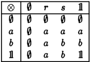
In the following, we choose to merge expert's opinions on each criterion first, and then to perform a mul ticriteria aggregation, since it might seem more nat ural to use the experts first to properly assess the score according to each criterion. Proceeding in the other way would assume that each expert is looking for a global evaluation of the candidate (may be using his own criteria aggregation attitude) and the decision maker is only there for combining and weighting ex pert's evaluations.Since we first merge the 1!'.d.f's, one of the allowable methods i s to use a weighted maxi mum. Indeed disjunctive combination is advisable in case of conflicting opinions ( Dubois and Prade, 1994], as it is the case here (conjunctive fusion can be applied only if there is no conflict). A disjunctive combination means that the opinion of an important expert will be taken into account, even if this can conflict with another important one. However, unreliable estimates should be discounted in the disjunction. The reliabil ity W;j attached to rr{ should be both upper bounded by the confidence a3 of DM in the expert j and the self-confidence /ij of the expert. This leads to take the weight Wij as the conjunctive-like combination of a j and /ij , Vi = 1, . . . , 6. The weighted disjunction is defined as:
As said above, W;j = Iii 0 a j where 0 is a conjunction operator from L-y x La to L-y. Table 5 defines 0 on the basis of an implicit commensurateness hypothesis of L-y and La.
| 0 | 0 | r | 8 | n |
|---|---|---|---|---|
| 0 | 0 | 0 | 0 | 0 |
| a | 0 | a | a | a |
| b | 0 | a | b | b |
| n | 0 | a | b | n |
Table 5: Definition of 0
| Wij | Mkt D | Fin D | Prod D | HR D |
|---|---|---|---|---|
| Ana | 0 | a | a | 0 |
| Lear | b | a | a | b |
| Exp | n | 0 | 0 | 0 |
| Com | n | 0 | 0 | b |
| Dec | a | a | a | a |
| Crea | n | 0 | 0 | b |
Table 6: Weights Wij for all criteria and directors Table 6 gives the weights for all criteria and experts. We apply formula (2) to 1!'.d.f's of Table 4, and obtain the 11' .d.f's of Table 5 (left).
We notice that some distributions are no longer nor malized (i.e., no score is fully possible at level n). This is because the weights are not normalized, i.e. VjWij < n for some i's, which means that the DM cannot be fully confident in any director when assess ing some criteria (namely Ana, Lear and Dec).
We should either use the unnormalized distributions to fully keep track of the problem, or normalize them in a suitable way. Here, we choose the second solution, and propose the following approach. We consider that the maximum of the distribution, denoted h, reflects the uncertainty level, considered to be -.h in the in formation. This means that the amount of conflict is changed into a level of uncertainty and the minimum level of the modified distributions will be -.h. Then, we make an additional hypothesis that the scale is a in terval scale (which is questionable!) so that the profile of the distribution is not changed. Specifically:
It means that + in (3) is defined by s; + Bj = Bmin(k+l,i+j) on a scale {so= 0, S!, ... , Sk, Sk+l = n}. The result is shown in Table 5. A slightly different method would be to keep possibility degrees equal to 0 at 0, since 11'1( s) = 0 means that all experts agree on the fact that the value s is impossible
| Ana | 0a0a0 | Ana | bnbnb |
| Lear | abbba | Lear | bnnnb |
| Exp | 000n0 | Exp | 000n0 |
| Com | 000n0 | Com | 000n0 |
| Dec | aaaaa | Dec | nnnnn |
| Crea | b000n | Crea | b000n |
The way of aggregating the criteria evaluations is not at all specified in the statement of the problem. Only qualitative levels of importance {3; are provided for each criterion i. Even with ordinal scales, different attitudes can be thought of. The aggregation may be purely conjunctive (based on "min" operation), or somewhat compensatory (using a median opera tion for instance). It might be also disjunctive: at least one important criteron is to be satisfied, it is modelled by a weighted maximum. More general ag gregation attitudes can be captured by Sugeno's in tegral ([Sugeno, 1977];[Grabisch et al., 1995]). Let us assume that the DM has a conjunctive attitude.
We use the weighted minimum method in what follows for the aggregation. With our notations, in the case of precise scores, the global score is obtained by
where V is a disjunctive operator from Ll' x L, to L,. Table 8 gives the definition of this operator.
| v | 0 | e | f | g | n |
|---|---|---|---|---|---|
| 1 | 1 | 2 | 3 | 4 | 5 |
| 2 | 2 | 2 | 3 | 4 | 5 |
| 3 | 3 | 3 | 3 | 4 | 5 |
| 4 | 4 | 4 | 4 | 4 | 5 |
| 5 | 5 | 5 | 5 | 5 | 5 |
The "fuzzy" evaluation provided by the 11' .d.f. 's can be handled in different ways. A natural manner to pro ceed is to extend multicriteria aggregation techniques to such non-scalar eva! nations (this can be done both if this step is done before or after the fusion step). At the technical level, this will be done using an extension principle [Zadeh, 1975] which enables to extend any function/operation f to any fuzzy arguments. Namely, j(P1, ... , Pm)(s) = V,=J(·'· . . ,,m)PI(s1)11 ... 1\Pm(s m ) where P;(s ; ) is the possibility degree of score si accord ing to 11'.d.f. P;. Here the result will be a possibility distribution 11' K restricting the possible values of the global evaluation of K. Then a fuzzy ranking method should be used for assessing to what extent it is cer tain, and to what extent it is possible that K 1 is better than K2, on the basis of 11'K1 and 11'K, in case of several candidates ([Dubois and Prade, 1983]).
Since scores of criteria are imprecise, the extension principle has to be used. We have for any s E L,
Applying this formula to our data, we finally obtain the distribution given in Table 9. The result can be
| score | 1 2 3 4 5 |
|---|---|
| possibility degree | b n n n o |
Note that if weighted min combinations are used both in the expert opinion fusion and in the multi-criteria aggregation then the two combinations commute.
6 General discussion
The reader may be astonished by the discrepancy be tween the results obtained by the belief function ap proach and by the possibilistic approach. This does not reflect any disagreement between the two ap proaches, but in fact two different options in the ag gregation mode of the criteria. Indeed, the TBM ap proach has used a compensatory aggregation mode, while weighted minimum has been used in the QPT approach (although it would be possible to use median operators in the qualitative setting in order to allow for compensation). The min-based combination is the only conjunctive idempotent attitude, whereas Demp ster's rule of combination is not idempotent (even though there exist other combination rules that are more 'cautious' and idempotent).
Moreover, when introducing the Goodness Score in the belief function approach, the underlying idea is that we are all the less demanding for reaching the maximum level of satisfaction as the criterion is less important. This is not at all the understanding chosen in the pos sibilistic approach (remember that the problem is not completely specified). Rather, the unimportant crite ria were considered as somewhat satisfied even if they were not at all satisfied.
In fact there are different possible ways of understand ing the weighting of the criteria, in a qualitative con junctive setting. Let c; (K) be the supposedly precise value of score of K, according to criterion i. Indeed, we can i) modify c;(K) into -,j3;Vc;(K) as we did, or
{ 5 if c;(K) 2:: ;3; ii) modify c;(K) into c;(K) if c;(K) < ;3; (;3; is interpreted as a threshold level to reach to be fully satisfied, taking advantage of the commensurateness hypothesis underlying Table 8). Choosing the option (ii) above in the QPT approach instead of (i) would be similar to the idea of Goodness Score as defined in the TBM approach.
Another difference is that the possibility distribution we have obtained represents the uncertainty pervading the genuine value of the candidate. It is not a scalar expectation, a thing which can be also computed in the possibilistic framework as explained now.
The assessment problem can be viewed as a decision to be made under uncertainty. Namely, the relevance of the criteria defines a candidate profile, i.e., a kind of utility function, while the value of the candidate K is ill-known with respect to each criterion (once expert opinions have been fused). Viewing the problem in this way, it is natural to compute to what extent it is cer tain (or it is possible) that the candidate K (whose level assessment may be pervaded with imprecision and uncertainty for each criteria) satisfies the criteria at the required level; see ([Dubois and Prade, 1995)) for an axiomatic view of the corresponding qualitative decision procedure. It corresponds to a fuzzy pattern matching problem ([Dubois et al., 1988]) in practice.
For each criterion i, we build a satisfaction profile Jli, e.g., Jl;(s) = -.;3; V s. Jli means that the greater the score, the better the candidate, and that the satisfac tion degree is lower bounded by -.;3; which is all the greater as i is less important. Then the certainty that K satisfies the profile is given by
where 11'c;K is supposed to be normalized. The possi bility that K satisfies the profile is
where 11'c , ( K ) has been obtained by fusing the expert opinions first, at the level of each criterion. The possi bility degree (very optimistic) should be only used for breaking ties in case of equality of the certainty de grees for different candidates. The aggregation by /\ ; of the elementary certainty and possibility degrees can be justified in the possibility framework (definition of a join possibility distribution of non-interactive vari ables ([Zadeh, 1975]), and interpretation of the global requirement in terms of a weighted conjunction of el ementary requirements pertaining to each criterion). The expression (6) and (7) can be viewed as possi bilistic "lower and upper expectations".
What is computed remains in the spirit of the ap proach detailed before. Instead of obtaining a pos- sibility distribution we obtain two scalar evaluations for which it should be possible to show that they sum marize this possibility distribution (in a sense to be made precise at the theoretical level). Anyway both approaches first compute the 11'c;(K)'s and are based on the choice of a weighted conjunction.
Lastly, it is also important to judge the (potential) explanation capabilities. Are the results provided by the system easy to explain to the user if neces sary? E.g., why the value of the candidate is fi nally assessed as such? Such explanation capabili ties are presented in [Farreny and Prade, 1992] and in [Xu and Smets,1996] for what concerns the QPT and the TBM, respectively.
For summarizing the main differences between the belief function (TBM) and the possibility-based ap proaches (QPT) on the value assessment problem, it is clear that the possibilistic method can handle poor data expressed in a qualitative, non-numerical, way whereas the belief function framework may more eas ily capture reinforcements and compensatory effects.
7 Concluding remarks
In this paper, we have taken advantage of a generic value assessment problem for discussing the different facets of the problem and raising the various difficulties and hypotheses which should be made at each step for computing a meaningful evaluation through two models, the QPT and the TBM.
The purpose of the paper was twofold: first identi fying and discussing various facets of a value assess ment problem, and second showing how two differ ent approaches (which have in common the capability of modelling imprecision) can handle the problem in manners which are in fact quite parallel.
The statement of the problem contains no number, but only ordinal assessments. Owing to the qualitative framework of possibility theory , the QPT provides an obvious solution. However note that it is important to consider the nature of the scales which are used in or der to know what operations are meaningful on them. Moreover commensurateness hypotheses are necessary.
With the TBM, numbers (the beliefs) are needed. They are in fact analogous to those a probability ap proach would ask for. The difference between the TBM and a probability approach is that the TBM accepts and uses the data just as they are, without introducing extraneous data. E.g., a probability ap proach would allocate (equal) probabilities to each of the individual values of the scores when the score is only known as a non-degenerated interval.
二
Sensitivity analysis can be performed, where either the values of the parameters (TBM) or the aggregation op erators ( QPT) are slightly modified and the robustness of the conclusions can be assessed. Furthermore the DM can also determine the sensitivity of the results if more precise data were collected,. Given this informa tion, the DM could efficiently ask to a specific expert to provide a better estimate of the candidate score for a specific criterion, avoiding getting "useless" data.
One important point in practice for this type of prob lem is also to be able to provide explanations to the user on the results. The qualitative framework of pos sibility theory allows for a logical reading and pro cessing of the evaluations. This offers a potential for explanation capabilities.
8 Acknowledgements
This work has been supported by the European work ing group FUSION (Esprit Project 20001: Fusion of Uncertain Data from Sensors, Information Systems and Expert Opinions). Special thanks are due to Si mon Golstein who helps stating the candidate value assessment problem considered in this paper.
References
- (Costa and Vansnick] Carlos A. Bana e Costa, Jean Claude Vansnick, A theoretical framework for measuring attractiveness by a categorical based evaluation technique (MACBETH). Xlth Int. Conf. on MCDM, August 1994, Coimbra, Portugal, 15-24
- (Dubois et al., 1997] Didier Dubois, Henri Prade and Regis Sabbadin, A possibilistic logic machinery for qualitative decision. Proc. of the AAAI'97 Spring Symp. Series on Qualitative Preferences in Delib eration and Practical Reasoning, Stanford, CA, March, 47-54, 1997.
- (Dubois et al., 1988] Didier Dubois, Henri Prade and Testemale, Weighted fuzzy pattern matching. Fuzzy Sets and Systems, 28(3), 313-331, 1988.
- (Dubois and Prade, 1983] Didier Dubois and Henri Prade, Ranking fuzzy numbers in the setting of possibility theory, lnf. Sci., 30, 1983.
- (Dubois and Prade, 1994] Didier Dubois and Henri Prade, Possibility theory and data fusion in poorly in formed environments. Control Engineering Prac tice, 2(5), 811-823, 1994.
- (Dubois and Prade, 1995] Didier Dubois and Henri Prade, Possibility theory as a basis for qualitative deci sion theory. Proc. of the 14th Inter. Joint Conf. on Artificial Intelligence (IJCA1'95), Montreal, Canada, 1924-1930, 1995.
- [Dubois and Prade, 1998a] Didier Dubois and Henri Prade, Possibility theory : qualitative and quan titative aspects, In Quantified Representation of
- Uncertainty and lmprecision(Ph. Smets eds. ), Vol. 1 of the Handbook of Defeasible Reasoning and Uncertainty Management Systems (D.M. Gabbay, Ph. Smets, series eds.), Kluwer Academic Publish ers, 169-226,1998.
- [Dubois et al., 1998b] Didier Dubois, Henri Prade and Regis Sabbadin, Qualitative decision theory with Sugeno integrals, in Proc. of the 14th Conf. Uncer tainty in Artificial Intelligence (UAI'98), Madison, July 24-26, 1998, Morgan Kaufmann, 121-128.
- (Farreny and Prade, 1992] Henri Farreny and Henri Prade, Positive and negative explanations of uncertain reasoning in the framework of possi bility theory, in Fuzzy Logic for the Managment of Uncertainty (L.A. Zadeh, J. Kacpryk, eds.), Wi ley, 1992, 319-333.
- (G r ab i s ch et a l . , 1995] Michel Grabisch, Hung T.Nguyen and Elbert A. Walker, Fundamentals of Uncer tainty Calculi with Applications to Fuzzy Infer ence, Kluwer Acad. Pub!., 1995.
- (Raufaste and Da Silva Neves, 1998] Eric Raufaste and Rui Da Silva Neves, Empirical evaluation of possi bility theory in human radiological diagnosis", in Proc. of the 13 th Europ. Conf. on Artificial In telligence (ECAI'98), Brighton, UK, Aug. 23-28, 1998, John Wiley & Sons, 124-128.
- (Shafer, 1976] Glenn Shafer, A mathematical theory of ev idence. Princeton Univ. Press. 1976.
- (Smets, 1993a] Philippe Smets, Belief Functions : the Dis junctive Rule of Combination and the Generalized Bayesian Theorem. International Journal of A p proximate Reasoning, 9 : 1-35, 1993.
- (Smets, 1993b] Philippe Smets, No Dutch Book can be built against the TBM even though update is not obtained by Bayes rule of conditioning. SIS, Workshop on Probabilistic Expert Systems, ( ed. R. Scozzafava), Roma, 1993, 181-204.
- (Smets and Kennes, 1994] Philippe Smets and Robert Kennes, The transferable belief model.Artificial Intelligence, 66 : 191- 234, 1994.
- (Smets, 1998] Philippe Smets, The Transferable Belief Model for Quantified Belief Representation. Hand book of defeasible reasoning and uncertainty man agement systems. Gabbay D. M. and Smets Ph. Eds. Vol. 1, Kluwer, Doordrecht, 1998, 267-301.
- (Sugeno, 1977] Michio Sugeno, Fuzzy measures and fuzzy integrals: A survey. In: Fuzzy Automata and De cision Process (eds.), North-Holland, 89-102,1977.
- (Xu and Smets,1996] Hong Xu and Philippe Smets, Some Strategies for Explanations in Evidential Reason ing Explaining the origin of a computed belief and finding which pieces of evidence are influencing the results. IEEE Transactions on Systems, Man and Cybernetics, 26A : 599-607, 1996.
- [Zadeh, 1975] Lotfi A. Zadeh, The concept of a linguistic variable and its application to approximate rea soning, Inform. Sci. Part 1, 8 (1975) 199-249; Part 2, 8 (1975) 301-357; Part 3 (1975) 43-80, 1975.