Belief Induced by the Partial Knowledge of the Probabilities

Philippe Smets IRIDIA

Universite Libre de Bruxelles Brussels-Belgium

Abstract:

We construct the belief function that quantifies the agent' beliefs about which event of Q will occurred when he knows that the event is selected by a chance set-up and that the probability function associated to the chance set up is only partially known.

Keywords: belief function, upper and lower probabilities.

1. INTRODUCTION.

1) The use of belief functions to quantify degrees of belief is muddled by problems that r e s u l t from the confusion between belief and lo w e r probabilities (or between plausibility and upper probabilities). Beliefs c an be induced by many types of information. In this paper, we consider only one very s p e c i a l case: beliefs induced on a frame of discernment Q when the clements of Q will be selected by a random process. It seems reasonable to defend the idea that the be l i ef of a n event should b e numerically equal to the probability of that event. This principle is called the Hacking Frequency Principle (Hacking 1965).

But there are cases where the p rob a b i l i ty function that governs the random process is not exaclly known. This lack of knowledge can be encountered when p r o b a b i l itics are partially defined or when data are missing. As an example, suppose an urn where there arc 100 balls. Its composition is not exactly known. All that is k n o w n is that there are between 30 and 40 black balls, between 10 and 50 white balls, and the other are red. What is your belief that the next randomly selected ball will be black? Suppose you have selected 50 ba l l s at random w i t h replacement and you have observed 15 black balls, 20 white, 10 reds and 5 'not black'. What is your belief now that there are between 35 and 37 b la c k balls? What is your belief now that the next randomly selected ball will be black? These are the problems we solve in this paper.

In this p a per, we accept that beliefs are quantified by belief functions, as described in the transferable belief model (Smets 1990b, Smets and Kennes 1994). The transferable belief model is a model for quantified beliefs developed independently of any underlying probabilistic model. It is neither Dempster's m od e l nor iL<; today versions (Shafer, 1990, Kohlas, 1994). It is n o t a model based on inner measures (Halpern and Fagin, 1990).

What we study here is just a special case of belief function. We study the belief induced by the knowledge of the existence of an objective chance set up that generates random events according to a probability function, probability function that happens to be only partially known to us.

1. Suppose a frame of d i s c e r n m e n t .Q, i.e., a set of mutually exclusive and exhaustive events such as one and only one of them is true (we accept the close world a ss ump t ion (Smets 1988)). Suppose the true element will be selected by a chance process. Let P:2 n �[O,l] be the probability function over n w h e r e P(A) for A<;;;Q quantifies the probability (chance) that the selected clement i s in A. We accept that this probability measure is "objective". The problem is to assess Your degree of belief. You denotes the agent who hold the beliefs. Your beliefs arc quantified by a belief function bel:2 n --7[0,1], about the fact t ha t the selected element is in A, given You only have some p ar tia l knowledge about the value of P.

Should You know P, t h e n by Hacking Frequency Principle (1965) Your degree of belief bei(A) for each A<;;; Q should be equal to P(A):

If You know that P(A) = PA VA C:Q

then bel(A) = PA VA C:Q

In that case bel is a probability function over Q. But remember that bel and P do not have the same meaning; they only share the same values. P quantifies the probability (chance) of the events in Q, bel quantifies the belief over Q induced in You by the knowledge of the value o f the probabilities. P exists independently of me; bel cannot e x i s t if You do not exist.

Let lP n be the set of probability functions over Q. Suppose that You know only that the probability function p that governs the random process over n is an element of a subset.:?-' of lP n· The problem is to determine Your belief about Q given You know only that Pis an element of.:?-'(but You do not know which one).

In many cases, !?' is uniquely defined by its upper and lower probabilities functions P* and P* where:

P*(A) =max { P(A) : Pe.'?-j = 1 - P*(A) or.91= (P: Pe!P0, P*(A) 5 P ( A ) 5 P*(A), VA<;;;Q}. Just as P and bel characterize different c on c e pts , P* a n d bel characterize also different concepts, even when P* is mathematically a belief function. The function bel concerns Your belief over Q. The function P* gives the lowest possible values for the pr o b a b i l i t y of the events in 0. c o m p a t i b l e with w h at You know.

This knowledge that Pe� IPn i s translated into a belief beliP n ov er IP0.1 That b e l i e f only supports .9, i .e . , its basic belief masses are:

Given Your belief over IP0, can You b u il d Your belief over Q, In this paper, we will show how t o build such a be l i ef function.

Classical material about belief functions and the tra n sfera bl e belief model can be fo u n d in Shafer (1976), Smets (1988) and Smets and Kennes (1994).

2. IMPACT OF HACKING FREQUENCY PRINCIPLE.

The general frame c o ns i s t s of :

• IP n: the set of probability f u n c t i o n s P over 0.;
• 0.: the f i n i te set of possible elementary e v e n t s Wj, i::: 1, 2 . . . n, (the outcomes of t h e stochastic experiment);
• -IBIP0: the set of belief functions over IP0.

Let N = [1, 2 ... n]. Let W = IPn x Q_ All subsets A of W can be r e p r es e n t ed as the finite union of the i nt e rse c t i on of A with each of the e l e m e n ta r y events Wi:

where Ai = proj(Ancyl(wi)Y:IPn. cyl(X) is t h e cylin­ drical e x te n s i o n of X on W where X denotes a subset of Q ( o r IP n). and proj(B) is the projection of Be;; W on Q (or IP n) ( c o n t e x t makes it clear which domain and which range are in v o lv ed).

The major problem solved in this p a per is the c on s tr u c t i o n of the belief function belw on W that would result if You were in a state of total ignorance about the value of P. If You have some prior b e l ie f bciiP n about the value of P, the belief belw over W would be combined with the vacuous extension of beliP 0 on W by the application of Dempster's rule of c o mb i n a t i on . We will treat essentially the c a s e where You only know that PE.:P where.9Z'is a subset of 1Pn. i.e., when.9'is the only focal

1 subscripts of m and bel d en ote their domain.

element and Your belief over lP n can be represented by the basic belief a s s i gn m e nt with miPn� = 1. G e nera l i z a t i o n for a finite (or countable) numbers of focal e le men t s is immediate. Further generalization is more deli ca t e .

Let IBw be t h e set of belief functions over W. What is their nature? We are going to construct the equivalent of the basic belief masses (bbm) on IBw. We say equivalent as W is not a finite space and the concept of basic belief masses has to be extended in order to cope with the structure of W. The bbm will become some sort of 'densities'. For simplicity sake, they are also denoted by m w : 2W�(O,I]. The value belw(A) is defined as the 'integral' of the mw values given to the non empty subsets of A. It ha p p en s that in the case co n s i d ere d in this paper, m w is a real density for which classical integrals are well defined. We call the mw f un c ti o n a basic belief density (bbd) to enhance its particular nature. T h o se subsets A of W such that mw(A)>O are called the fo ca l elements of mw.

The first co n s tr a i n t about mw results from Hacking Frequency Principle. Suppose You know the values P(Wi) of the o bj e c t i v e probability function P on Q for every WjE Q (what is translated by .9 = {P}). Let beln{Pl denotes Your belief over 0. when You know that .9 = {P].2 By H a ck i n g Frequency P ri n c i p le , the value bcln ( P) (X) for any subset X of Q is numerically equal to the probability P(X) given to X.

By c o n s t r u ct i o n , beln {P) re s u l ts from the marginalizing ofbclw{PJ o v e r 0.:

Hacking Fr e q u e n c y P r in c i ple i m p l i e s th e n e x t re q uire me n t .

Let n(P) = cyl( {P)) <;;;; W, t h e n n(P) =: u ( {P(�)}, Uli) by tEN 2.1. T h u s belw { P l(cyl(X)) = belw(cyl(X)I1t(P)). The s eco n d term is just the result of the conditioning of belw o n c y l ( {P} ) , what i s achieved by the application of Dempster's rule of conditioning. Hence the bbd mw(A), A .;;;w is transferred to Ann:(P). Let A= u (Ai, w{)CW, ieN then m(A) is transferred to Ann(P) = u (Ain {P(Uli)), iEN

Wj).

2Superscripts of bem and m denote Your knowledge about P, i.e., the focal element of be!IP n ·

The result of this conditioning on rt(P) is a probability f u nc t i on . Hence b e l w {P} must be a Bayesian belief function, i.e., only singletons can be focal elements and beiw iPl (W) = 1. The singletons of W have the form ({P(Wi)J, Wi) for ie {1, ... n}, Pe 1Pn,. Hence mw must satisfy:

The impact of Hacking Frequency Principle, translated by 2.3, i s very strong. It implies that the focal elements of mw can be r e p r e sent e d as u (Aj, Wj) where the Aj, ieN

i=l , ... n, are non empty elements of a partition of IP n·

3. THE CASE WHERE IQI = 2.

We study now the case where IQI = 2. Let n = {S, F) where S and F denote Success and Failure, respectively.

0

a

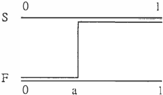
Figure 1: Structure of the domain of mw and one e x am p le of bbd centered on a when 101 = 2.

Let A r:;;, W be a focal e le m e nt of mw, then A = (a, S)u( a, F) w h e r e a.qo, 1] and a is the complement of a. r e l a t iv e to [0, 1]. For simplicity sake, the bbd m w (( a , S)u( a, F)) is written as mw(a.).

W can be graphically represented by two [0, 1] intervals where the upper [0, 1] interval is the i n t e r se c t i o n of W with S, and the lower one is the intersection of W with F (see f ig u r e 1). Every focal element of mw is made of a set of mutually exclusive and exhaustive intervals that are either in the S domain or the F domain. By co n v e n t i o n , intervals are defined as closed to the left and open to the right, except when 1 is the r i g h t limit, in which case the interval is also closed to the ri g h t .

We introduce an extra assumption.

for every o��b�c�d� 1.

It is equ iv al e n t to assuming that mw(a) is null except if a = (a, 1]. Th e origin o f t h e a s s u m p t io n is to be found in th e meaning of the bbd. The bbd mw(a) for � [ 0 , 1] i s that part o f belief (a density here) that supports the fact that P(S)e a (and P(F)e a). Suppose we co ndi ti o n mw on S. Each bbd mw(a) is transferred to (a, S)r;;,w. Requirement 2 means that if after conditioning on S a bbd supports P(S) = x e [0,1], it also supports every value in [0, 1] larger than x. Observing a success could support P(S) = .3, b u t that support should then also be given to P(S) = .4 etc ....

This assumption means that each focal element is a step function that starts from ({0). F), jumps from the F domain to the S domain at some a in [0,1], and ends at ( { 1 J, S) (see figure 1).

Finally, if we apply again the Hacking Frequency Principle, we obtain after conditioning on 9= {P) with P(S) = p, P(F) = 1-p:

The second equality results f r om the f a ct that only those bbd that jump before p will touch ( {p}, S) and bcJ n {Pl (S) is equal to the integral of those bbd that touch ( { p}, S). Derivating both terms on p implies that:

In c on c lus i o n we have derived the bbd on w w h e n IQI = 2.

Some properties can be easily derived.

1. Suppose the agent knows that.9'= {P: a::; P(S)::; b, 0 �a < b � I}. We condition mw on the c y l ind r i c a l extension of [a, b). The bbd mw(A) f o r Ar;;,w is transferred to A n cyl( [ a , b)). bel v/'t S) is the integral of a l l the bbd that touch only S after conditioning on cyl((a, b]), i.e., those bbd that j u m p to S be for e a:

Similarly pl w9t S) is the integral of all the bbd that touch S, i.e., that j u m p to S b e f or e b:

This result should not be extrapolated blindly to higher dimensions (see section 4 ).

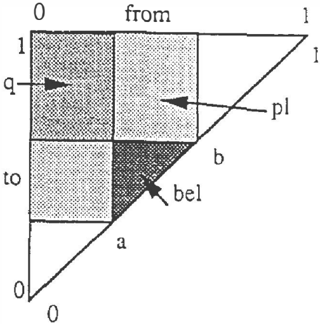
1. The case IQI = 2 can be nicely represented by f i g u r e 2 (Smets, 1978). Each point in the triangle corresponds to one interval of ( 0 , 1 ] . In g en e r al, if p os iti v e bbd are given

only to intervals, we assign t h e bbd g i v e n to [a,b] to the point (a,b) of the triangle. Then:

The result of the application of Dempster's rule of combination is given by mu l t i p l yi n g the commonality functions.

0

Figure 2: P a r a me tric representation on beliefs on [0, I] when the focal elements are int e r v a l s . The shaded areas are those on which int e g r a ti o n is pe rf o r me d in order to compute bel([a,b] (a triangle) , q([a,b]) (a rectangle ) and pl([a,b]) (a rectangle with right lower corner truncated).

In the present case (1.0.1=2) the non-null bbd of mw ob ta i n ed after conditioning on S are g iven to the intervals [a,l], h e n c e they c l u s ter on the upper horizontal line. Those obtained a f te r conditioning on F arc g i ve n to the i n t e r v a l s [O,b], h e n c e they cluster on the left vcnical linc.

Suppose You p e r f o r m n i n de p e n d en t experiments and ob s e r v e r successes, s failures w h er e r + s � n (the di ff e r e n c e n -(r + s) is the number of experiments for which the outcome is not available). The commonality f un c t i o n induced on [f' n = [0, I]

• -by a success is: q!P n( [ a, b] I S) = a -by a failure is: q!P , /[a,b] I F)::::: 1-b -by a 'SuF' is: q!Pn([a,b] I SuF) = 1

The belief function induced by 'SuF' is the vacuous belief f u n ctio n that reflect th e state of total ignorance i n which You are after just learning the tautology 'SuF'. He n c e we can j u st as well drop all 'vacuous' results and assume n = r+s.

The commonality function induced by r successes and s failures in n independent ( B e m o ul l i a n ) trials is o b ta i n e d by multiplying the c o rre s p o n d i n g commonality functions. Hence:

In t h a t case, by d e r i v a tin g q!P n ([a,b) I r, s ) an d appropriate normalization, we get:

where r

When n�oo, r�np, s--tn(l-p) (hence p = lim...!..._), the r+s limit of m([a,b] I r, s) t en d s to 0 except for a dirac function at p. In t h a t case bel(A I r,s) = I if pEA and 0 otherwise. A ft e r accumulating an infinite number of information, You will be in a state of 'total c erta i nt y ' , of 'knowledge' about the value of P(S).

3) S upp o s e You want to compute the belief that the next outcome is a success (or a failure) given You have already observed r successes and s failures in n independent trials. We use m([a,bJ I r, s) as the a priori belief over [0, 1]. Dempster's rule of combination m12 ::::: m16;)m2 can be represented as (Dubois and Prade, 1986, SmeL<>, 1993a):

where m1 (A I B) and b e l 1 (A I B) are unnormalized conditional basic belief m a ss e s and b e l i e f functions. Generalizin g this relation in the present context and denoting beln(P: P(S)e (a,bll(S) by beln(S I P(S)E[a,b]) (which value equals a), one obtains:

This result shows that the observed proportion is an excellent approximation of beln if r+s is n o t too small.

4. CASE WITH IQI = 3.

Suppose 1!11 = 3 where n = {A, B, C}. 1P n can be represented by an equilateral triangle where each point corresponds to an element of 1P n . The three heights are equal to the three probabilities P(A), P(B) and �(C): Th _ e he i gh t of such a tr i an g l e is 1 and the length of 1L<; s1de IS equal to -f413.

By r e qu i r e m ent 1, we know th a t the focal elements of mw can be represented by:

where (9'-'A, .9E, �) a r e the elements of a p a r t it i o n of !P n .

In order to s p ec i f y the f o r m of the subsets_9X, XE (A, B, C}, we consider the conditioning of mw on the s c t .9'i c: IPn where

where bo ,a1 E [0, 1], bo < 1-aJ.

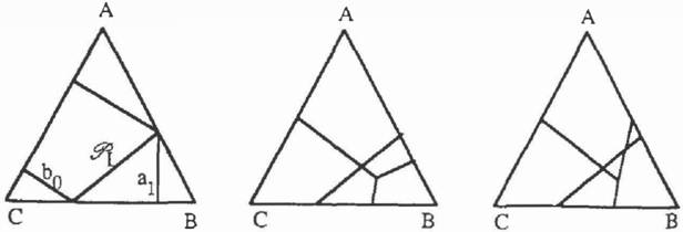
This set .9'L corresponds to the subset of 1P n w h e r e P(A)E [0, ai] and P(B) and P(C) a r e l i n e a rl y related to P(A). Requirement 3 states that, after conditioning mw on.9i, the bbd so obtained on the s p a c c .9-L is identical to those obtained when 101=2 (indeed every clement of the n ew subdomain is characterized by P(A) as when IQ1=2). T he r e f or e after further conditioning on A, the focal elements on.9L should be of the form of intervals [a, a1l (see figure 3). This requirement is s uf f i c i e nt in order to d er iv e the structure of the focal elements of mw.

Requirement 3:

If IQJ = 3, for every fTA. there exists an aE [0, a I) su c h that t h e projection of .9'A on .9i is the interval [a, a1l·

Requirement 3 can identically be defined as:

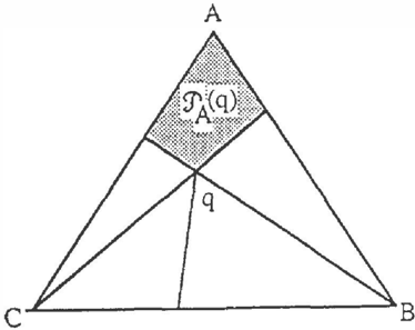
Ea c h r equir eme n t implies that the limits between.9'A and .913 must be a straight line passing through the corner where P(C) = 1 and that crosses the opposite side of the triangle (and similarly for the other limits). Every focal clements of mw can be labeled by an e l e m en t q = (qA, qs, qc)e IP n . The focal element labeled by q is the set

and similarly for ,9Js(q) and �(q) where the A,B,C­ indcxes are s y m m et r i c a ll y exchanged. The graphical representation of .9'A (q) is the upper corner of the 1P n triangle that i n c l u d e s all poi nts in IP n between the upper corner and the two straight lines drawn from the tw o other corners through q. belw(X l A) for Xt.;;;IPnwill be the ' i nte g r a l ' of all the bbd given to the focal elements .9\q) such that Xc:.9-'A(q).

F i g u r e 4 shows the structure of the partition so generated.

The v a l u e of bcl n (A 1.:1'= {(a, b, c)} ) is the ' i n te g r a l ' of mw taken over all q in the triangle which corners are (0, 0, 1), (0, 1, 0) and (a, b, c). Reapplying the Hacking F r e q ue n c y Principle we have:

It can then be proved that the only function mw s y m m e t r i c in the three arguments o f q that satisfies (4.3) for every (a, b. c) E IP n is the function mw(.9'{q)) = {3 for every qE IP n ·

Some properties derived from this solution arc detailed.

1. Iff?-'= [(.5, 0, .5), (.5, .5, 0)}, then mn(A) = l/3, mn(B) = mn(C) :::: 0, m.n(AuB) :::: mn(AuC) = l/6, mn(BuC) = 1/3, mn(AuBuC) = 0. This result merits some reflection. One might be s u rp r i sed that even though P(A) :::: .5 is exactly known, one does not have beln(A) =
2. .5. If the frame had b e e n A versus A, the critic would have been appropriate, except th a t in such a f r a m e we just have the required r e s u l ts . The difference observed here reflects the fact that there are t h re e clements. What is n i c e is that the pignistic probability induced in this case is s uc h that BetP(A) = .5 (the p i g n i s t i c transformation is detailed in next section).
3. If§-1= {(.5, b, c): b+c = .5], then mn(A) = I/3, mn(B) = mn(C) = 0, m.n(AuB) = mn(AuC) = l/6, m n ( B u C) = 1/4, mn(AuBuC) = 1/12. The same remarks hold as for t he case 1, but BetP(A) = .5 as it should.

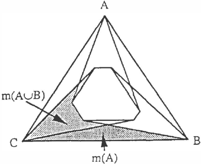
1. Suppose You know that §-lis characterized by a lower probability f u nc t ion P* on .n. Let P * be the upper probability function dual of P*, i.e., P * (X) = 1 P .. (X) for X�Q. Let a= P*{A), b = P*(B), c = P*(C), A= P*(A), B = P*(B), C = P*(C). The belief on Q induced by the set &?.'of probability distributions P on .n compatible with the upper and lower probabilities (i.e., VA c:::n, P ... (A):S:P(A):-;;?*(A)) is g iv e n by:

These results are obtained by computing the various surfaces d e s c r i be d in figure 5.

It is worth noticing that bel i s not equal toP*, even when P* is a belief function. Why should they? The transferable belief model never requires that the belief function that quantities our belief should be the lower e nv el o p of a set of probability function.

5. PIGNISTIC PROBABILITY.

In Smets (1990a, 1993b) an d Smets and Kennes (1994), we have shown how to build the appropriate probability function BclP, called the pignistic probability function, from a belief function when a decision must be made. We have shown that the only 'rational' transformation, called the pignistic transformation, must satisfy the following r u l e when the b e t t i n g frame Q is finite. Let m be the basic

belief assignment quantifying the agent's beliefs over n. For roe.Q,

where IAI is the number of elements of Q in A. Any other probability function would lead to irrationality in the betting behavior of the agent. Its extension to continuous cases is easy to realize if the bbd are really densities, in which case sums become classical integrals.

We study how decision should be made when beliefs are induced by a set of probabilities, i.e., how to derive the appropriate pignistic probability from the i n i t ia l be lief induced by the knowledge that Pe� IP Q· The choice of the appropriate betting frame is important. We could think to build the belief function over Q that quantifies our belief over Q and apply the pignistic transformation to such a belief function over Q using Q as the betting frame. But this is an erroneous strategy as the betting frame is not Q but W. The beliefs induced by Pe .9' i s a belief over W, the belief derived on Q is only the result of the marginalization of the first one on n.

Using W as the betting frame, we apply the pignistic transformation to Belw. For X<: IP n let S(X) b e the surface of X. Suppose the agent who wants to bet on Q knows only that PE .9: The pignistic transformation implies that the bbd mw(.:?-{q)) given to j'{q) (see (4.2)) be equally distributed among the elements of :7'.

Interchanging the order of integration, one gets that

where

One has:

I(X)

=

1 if X:;e0, 0 otherwise.

hence:

The pignistic probability BetPn(A) so derived is equivalent to the probability o n e would derive by assuming an equi a priori density over rPn. conditioning it on 9, and computing the expected probability of P(A).

These are quite natural results. B et P n ( . I .9) indeed happens to be the center of gravity of§-'", but its dcri vat ion does not result from the use of an equi a priori density over !P n· It just happens that both approaches lead to the same results: 1) t h e equi a priori density over !Pn and 2) the application of the pignistic transformation combined with the evaluation of BetP n(X I� as Bet.Pw(cyl(X) 1.97 for X<: Q, where BetPw is the pignistic probability obtained from belw(. IYj over the betting frame W.

6. CONCLUSIONS:

1. Generalization to 1.01 > 3 is conceptually easy, but very laborious when solutions must be written down. Nothing new comes out of it. In practice, computation will not been based on the explicit equations, but on some Monte Carlo method.
2. Generalization of the procedure can be achieved if one has a non-degenerated belief function on !P Q if there are only a finite number of subsets of !P n that receive positive basic belief masses (more general cases are not considered here). Let (.;?-l1: i= 1, 2 ... n} be the set of focal elements of beliP n with their basic belief masses miP0�). For each focal element.q', we derive belw(. I PE�) over W. The belief function belw over Q induced {(.:1-i. miP0�)): i= l, 2 . .. n)is:

1. Suppose two pi e c e s of evidence that say that Pe§-'1 and PE.0'2, respectively. The combination of these two pieces of evidence leads to the knowledge Pe.9'ln9'2·

One could build bell on W as the belief function induced by the knowledge that Pe.99.. Identically, one could build bel2 on W as the belief function induced by the knowledge that Pe.9'2. One could then be tempted, erroneously in fact, to combine bel 1 and bel2 into bel1 EBbel2 by Dempster's rule of combination.

One could also build bel12 on W as the belief function induced by t h e knowledge that PE.9'1 rl9'2. In general bcl12 ;<:bell (Bbel2. Only bel 1 2 is correct. Indeed Dempster's rule of combination is applicable iff both pieces of evidence are distinct, and distinctness is not satisfied in the present context because of the existence of a unique underlying probability function on Q that create a link between the two pieces of evidence.

1. In conclusion, the knowledge that the probability function P over n belongs to some subset .9' of IP n permits the construction of a belief function bel over IP n x Q and over n. It must be enhanced that in general the belief function beln induced over Q by a lower probability function P"' will not satisfy beln = P* even if P* h a p p e n s to be a belief function. By showing what is

the belief induced by a lower probability, we hope we have been able to show the fundamental difference between the upper and lower probabilities model and the transferable belief model (see also Smets, 1987, Smets and Kennes, 1994, Halpern and Fagin, 19 9 0).

Acknowledgment: Research work has been partly supported by the Action de Recherches Concertees BELON funded by a grant from the Communaute Fran.;:aise de Belgique and lhe ESPRIT III, Basic research Action 6156 (DRUMS II) funded by a grant from th e Commission of the European Communities.

Bibliography:

DUBOIS D. and P RA D E H. (1986) On the unicity of Dempster rule of combination. I n t . J. Intelligent Systems, 1:133-142.

HACKING I. (1965) Logic of s tat i s ti c a Cambridge University Press, Cambridge,

HALPERN J.Y. and FAGIN R. beleif: beleif as ge n e ra li zed probability and belief as evidence. submitted for publication.

l inference. U.K. (1990) Two views of

KOHLAS J. and M O NNE Y P.A (1994) Representation of Evidence by Hints. in Advances in the D e m p s t c r ­

Shafer Theory of Evidence. Yager R.R., Kacprzyk J. and Fedrizzi M., eds, Wiley, New York, pg. 473-492.

SHAFER G. (1976) A mathematical t h eor y of evidence. Princeton Univ. Press. Princeton, NJ.

SHAFER G. (1990) Perspectives in the theory and practice of belief functions. Intern. J. Approx. Reasoning, 4:323-362.

SJ.\1ETS Ph. (1978) Un mo d e l e mathematico-statistiquc simulant le processus du diagnostic medical. Doctoral dissertation, Universite L ib re de Bruxelles, Bruxclles, (Available t h r o u g h U ni v e r s i t y Microfilm International, 30-32 M o r ti m e r Street, London WIN 7RA, thesis 8070,003)

SJ.\1ETS P. (1987) Upper and lower probability f un c t i o ns versus belief f u n ct i on s . Proc. Int e rn a t i o n a l Symposium on Fuzzy Systems and Knowledge Engineering, Guangzhou, China, J u ly 10-16, pg 17-21.

SJ.\1ETS Ph. (1988) Belief functions. in SMETS Ph, MAMDANI A., DUBOIS D. and P R AD E H. eel. Non standard logics for automated reasoning. Academic Press, London p 253-286.

SJ.\1ETS Ph. (1990a) Construucting the pignistic probability f u nc t i o n in a con t e x t of uncertainty. Uncertainty in Artificial Intelligence 5, Henrion M., Shachter R.D., Kana! L.N. and Lemmer J.F. cds, North Holland, Amsterdam, , 29-40.

SMETS Ph. (1990b) The c o m b i n a ti o n of evidence in the transferable belief model. IEEE-Pattern analysis and Machine Intelligence, 12:447-458.

SJ.\1ETS P. (1993a) Belief functions: the d i s j u n c t i v e rule of combination and the generalized Bayesian theorem.

Int. J. App ro x i m at e R e as o ni n g 9:1-35.

SMETS P. (1993b) An axiomatic justifiaction for the use of belief function to quantify beliefs. DCAI'93 (Inter. Joint Conf. on AI), San Mateo, Ca, pg. 598-603. SMETS Ph. and KENNES (1994) The transferable belief model. Artific ial I n te l l i g e n c e, 66:191-234.

Ignorance and the Expressiveness of Single- and Set-Valued Probability Models of Belief

Paul Snow

P.O. Box 6134 Concord, NH 03303-6134 USA [email protected]

Abstract

Over time, there have been refinements in the way that probability distributions are used for representing beliefs. Models which rely on single probability distnlnrtions depict a complete ordering among the propositions of interest, yet h uman beliefs are sometimes not completely ordered. Non-singleton sets of probability distributions can represent partially ordered beliefs. Convex sets are particularly convenient and expressive, but it is known that there are reasonable patterns of belief whose faithful representation require less restrictive sets. The present paper shows that prior ignorance about three or more exclusive alternatives and the emergence of partially ordered beliefs when evidence is obtained defy representation by any single set of distributions, but yield to a representation based on several sets. The partial order is shown to be a partial qualitative probability which shares some intuitively appealing attributes with probability distributions.

1. INTRODUCTION

Probability distributions have long been advocated as a useful foundation for the modeling of beliefs. The best known form of probabilistic belief representation consists of a single distribution. Such models bring with them a well-developed normative theory of behavior in the face of risk (Savage, 1972) which has had many adherents over the years.

Recently, some r esearc hers have concluded that single distribution models are too restrictive. Beliefs may not always be completely ordered by the believer, even though a single probability distnbution necessarily represents them as being so. Nevertheless, other attributes of probability distributions do seem like accurate portrayals of how beliefs behave with respect to Boolean combinations of the underlying events, and of how beliefs change in the f8ce of evidence. Some of these desirable attributes are peculiar to probability distributions. So, to have the attnbutes, a belief representation must either use probability distributions or else use measures that agree with some probability distributions (Snow, 1992).

One way to get the desirable attributes of probabilities without the undesirable restrictiveness of a compJete ordering is to model beliefs using non-singleton sets of probability distributions. It is often convenient to use convex sets of probability distributions, which arise as solutions to systems of simultaneous linear inequalities. Many natural language expressions of belief are easily translated into linear inequality constraints (Nilsson, 1986), e.g. "This event is at least as likely as that one." Linear constraint systems can be revised simply by Bayes' formula (Snow, 1991). Although there is a diversity of opinion about how set estimates might inform decision making, there are useful suggestions for decision rules in the literature (for a review, see Sterling and Morren, 1991).

As versatile as convex sets are, there are reasonable belief patterns that convex sets fail to represent. For exam ple, the set of posterior probabilities derived from a convex set of priors and a convex set of conditionals is g en erally not convex (White, 1986). Further, some important constraints are non-linear. Kyburg and Pittarelli (1992) discuss the non-convex sets which arise from the non­ linear assumption of independence between events.

The present paper explores a circumstance where no single set of probability distributions, convex or otherwise, faithfully rep resen ts a reasonable pattern of belief: namely, ignorance being overcome by evidence when there are more than two alternatives. By ignorance, we mean that the believer is unwilling to · assert any non-trivial prior ordering among the sentences of interest. By being overcome by evidence, we mean that the believer will assert some non-trivial orderings if the contrast between the conditional probabilities for the evidence given the sent en<:es is sufficiently impressive.

A probabilistic solution to the representation of ignorance being overcome by evidence is presented. Although the model is more complex than a single set of probability

distributions, the orderings that arise have much in common with single posterior probability distributions, and inference about the orderings is computationally inexpensive.

2. NOTATION AND ASSUMPTIONS ABOUT IGNORANCE

In this paper, we sball use the notation

to denote the condition that the believer asserts that sentence S is, with a warrant satisfactory to the believer, at least as belief �worthy as sentence T in light of evidence e. If evidence e does not lead the believer to assert an ordering of sentences S and T, then we write

The condition of having no relevant evidence is indicated by the particle nil, as in

which expression denotes that there is no ordering between some sentences S and T in the absence of evidence.

We shall assume that the sentences of interest belong to a partitioned domain, which is defined as f ollows;

Definition. A partitioned domain is a set comprising:

• (i) the always-true sentence, denoted true
• (ii) the always false sentence, denoted false
• (ill) two or more mutually exclusive sentences, called atoms
• (iv) well-f ormed expressions involving atoms, or, and parentheses, called simple disjunctions

(v) well-f ormed expressions involving simple dis junctions, true, f alse, or, not, and parentheses

We shall assume throughout that the atoms in the domain are collectively exhaustive, that is, one of the atoms is true. This additional assumption places little epistemological burden on the believer (at worst, it means that one of the atoms is "none of the other atoms are true"), and has the convenient eff ect that every sentence in the domain has an equivalent simple dis junction. Finally, although infinite domains are useful in such applications as statistical hypothesis testing, we shall assume throughout this paper that the number of atoms in the domain is finite.

Our first assum ptions about ignorance, and the conquest of ignorance by evidence express the f ollowing ideas. If no evidence has yet been observed, and the question of relative belief -worthiness is not answerable on logical grounds, then there is no satisfactory warrant to order one sentence ahead of another. Even after evidence has been observed, the question may remain open. Once a commitment to an ordering is made, then other commitments may be inf erred by conditional probability considerations. A belief -ordering consistency principle discussed by Sugeno (unpublished dissertation, cited in Prade, 1985) obtains regardless of the presence or absence of evidence. The f ormal assumptions are:

AI. (Lack of explicit non-trivial prior orderings) For any sentences S and T,

Al. (Lack of implicit non-trivial prior orderings) Values for conditional probabilities and orderings among them are neither known nor assumed if those values or orderings imply non-trivial constraints on the prior probabilities.

AJ. (Consistency) For all evidence e, including nil, and any sentences S and T,

A4. (Impartiality) If S >e> T, and S' and T' are sentences, and S is exclusive ofT , then

• AS. (Recovery from ignorance about atoms) For exclusive atoms s and t, and non-nil evidence e, a neceswy condition f or s >e> t is that p( e I s ) >= p( e I t ), and if p( e t s ) > 0, then the inequality is strict. If p( e I s ) > 0, then p( e I t ) = 0 is not a necessary condition f or s >e> t.
• A6. (Dominance) For any sentences S, T, U and U where (S and U) and (T and U) are both f alse and U implies U, and f or all evidence e, including nil,

3. COMMENTARY ON THE ASSUMPTIONS

Assumption Al explains one circumstance where we decline to assert any ordering: when there is no evidence, and the one sentence doesn't imply the other. A2 restricts the scope of the assumptions to problems whose givens rule out no prior probability distribution over the atoms. The conditions in assumption A2 reflect the easily-shown f act that a dis junctive conditional like p( e I S ) is a convex combination of the conditionals f or the atoms in S, with weights proportional to the prior probabilities of the atoms.

Assumption

A3 says that we always assert an ordering