Best-First AND/OR Search for Most Probable Explanations

Radu Marinescu and Rina Dechter

School of Information and Computer Science University of California, Irvine, CA 92697-3425 { radum,dechter } @ics.uci.edu

Abstract

The paper evaluates the power of best-first search over AND/OR search spaces for solving the Most Probable Explanation (MPE) task in Bayesian networks. The main virtue of the AND/OR representation of the search space is its sensitivity to the structure of the problem, which can translate into significant time savings. In recent years depth-first AND/OR Branch-andBound algorithms were shown to be very effective when exploring such search spaces, especially when using caching. Since best-first strategies are known to be superior to depth-first when memory is utilized, exploring the best-first control strategy is called for. The main contribution of this paper is in showing that a recent extension of AND/OR search algorithms from depth-first Branch-and-Bound to best-first is indeed very effective for computing the MPE in Bayesian networks. We demonstrate empirically the superiority of the best-first search approach on various probabilistic networks.

1 INTRODUCTION

Belief networks [1] are a class of graphical models that provide a formalism for reasoning about partial beliefs under conditions of uncertainty. They are defined by a directed acyclic graph over nodes representing random variables of interest. The arcs signify the existence of direct causal influences between linked variables quantified by conditional probabilities that are attached to each cluster of parentschild nodes in the network. The Most Probable Explanation (MPE) task in belief networks calls for finding a complete assignment to the variables having maximum probability, given the evidence. It is typically tackled with either inference or search algorithms [1, 2, 3].

The AND/OR search space for graphical models [4] is a framework for search that is sensitive to the independencies in the model, often resulting in reduced search spaces. The impact of the AND/OR search to optimization in graphical models and in particular to the MPE task was explored in recent years focusing exclusively on depth-first search.

The AND/OR Branch-and-Bound first introduced by [3] traverses the AND/OR search tree in a depth-first manner. The memory intensive Branch-and-Bound algorithm [5] explores an AND/OR search graph, rather than a tree, by caching previously computed results and retrieving them when the same subproblems are encountered again. The depth-first AND/OR search algorithms were shown to outperform dramatically state-of-the-art Branch-and-Bound algorithms searching the traditional OR space.

In a recent paper [6] we introduced best-first AND/OR search algorithms for solving 0-1 Integer Programming problems, and demonstrated that, given enough memory, they are superior to Branch-and-Bound algorithms we developed earlier [7]. Subsequently, in [8] we extended this approach for Weighted CSP (WCSP) problems when using best-first AND/OR search guided by bounded mini-bucket heuristics. We demonstrated, again, that the best-first algorithms are more efficient than their Branch-and-Bound counterparts for various hard WCSP benchmarks.

In this paper we shift our attention to probabilistic networks, focusing on the MPE tasks. The extension of bestfirst AND/OR search from WCSP to Bayesian networks is straightforward. Hence, the main contribution of the current paper is in its empirical evaluation of the scheme over a wide range of probabilistic networks, including random networks, coding networks as well as hard instances from genetic linkage analysis. We show that this class of algorithms improves on the most competitive complete MPE solvers, thus it can potentially push the landmark of computation further, assuming memory is available.

The paper is organized as follows. Section 2 gives background on belief networks and AND/OR search spaces. Section 3 describes the best-first AND/OR search algorithm. Section 4 presents an extensive empirical evaluation and Section 5 concludes.

sent partial assignments. This search space does not capture the structure of the underlying graphical model. However, to remedy this problem, AND/OR search spaces for graphical models were recently introduced by [4]. They are defined using a backbone pseudo-tree [9].

DEFINITION 3 (pseudo-tree) Given an undirected graph G = ( V, E ) , a directed rooted tree T = ( V, E ′ ) defined on all its nodes is called pseudo-tree if any arc of G which is not included in E ′ is a back-arc, namely it connects a node to an ancestor in T .

AND/OR Search Trees Given a belief network P = 〈 X,D,F 〉 , its primal graph G and a pseudo-tree T of G , the associated AND/OR search tree, denoted S T , has alternating levels of OR nodes and AND nodes. The OR nodes are labeled X i and correspond to the variables. The AND nodes are labeled 〈 X i , x i 〉 and correspond to value assignments in the domains of the variables. The root of the AND/OR search tree is an OR node, labeled with the root of the pseudo-tree T .

The children of an OR node X i are AND nodes labeled with assignments 〈 X i , x i 〉 , consistent along the path from the root, path ( X i , x i ) = ( 〈 X 1 , x 1 〉 , ..., 〈 X i -1 , x i -1 〉 ) . The children of an AND node 〈 X i , x i 〉 are OR nodes labeled with the children of variable X i in T . Semantically, the OR states represent alternative solutions, whereas the ANDstates represent problem decomposition into independent subproblems, all of which need be solved. When the pseudo-tree is a chain, the AND/OR search tree coincides with the regular OR search tree.

A solution tree Sol S T of S T is an AND/OR subtree such that: (i) it contains the root of S T ; (ii) if a nonterminal AND node n ∈ S T is in Sol S T then all its children are in Sol S T ; (iii) if a nonterminal OR node n ∈ S T is in Sol S T then exactly one of its children is in Sol S T .

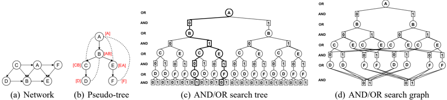
EXAMPLE 1 Figures 1(a) and 1(b) show a belief network and its pseudo-tree together with the back-arcs (dotted lines). Figure 1(c) shows the AND/OR search tree based on the pseudo-tree, for bi-valued variables.

Weighted AND/OR Search Trees The arcs from OR nodes X i to AND nodes 〈 X i , x i 〉 in the AND/OR search

2 BACKGROUND

2.1 Belief Networks

DEFINITION 1 (belief network) A belief (or Bayesian) network is a quadruple P = 〈 X,D,F 〉 , where X = { X 1 , ..., X n } is a set of variables over multi-valued domains D = { D 1 , ..., D n } . Given a directed acyclic graph DAG over X as nodes, F = { P i } , where P i = { P ( X i | pa ( X i )) } are conditional probability tables (CPTs for short) associated with each variable X i , and pa ( X i ) are the parents of X i in the acyclic graph DAG . A belief network represents a joint probability distribution over X , P ( x 1 , ..., x n ) = ∏ n i =1 P ( x i | x pa ( X i ) ) . An evidence set e is an instantiated subset of variables. The moral graph (or primal graph) of a belief network is the undirected graph obtained by connecting the parent nodes of each variable and eliminating direction.

Acommon optimization query over belief networks is finding the Most Probable Explanation (MPE), namely, finding a complete assignment to all variables having maximum probability, given the evidence. A generalization of the MPE query is Maximum a Posteriori Hypothesis (MAP), which calls for finding the most likely assignment to a subset of hypothesis variables, given the evidence.

DEFINITION 2 (most probable explanation) Given a belief network and evidence e , the Most Probable Explanation (MPE) task is to find an assignment ( x o 1 , ..., x o n ) such that: P ( x o 1 , ..., x o n ) = max X 1 ,...,X n ∏ n k =1 P ( X k | pa ( X k ) , e ) .

The MPE task appears in applications such as diagnosis, abduction and explanation. For example, given data on clinical findings, MPE can postulate on a patient's probable afflictions. In decoding, the task is to identify the most likely message transmitted over a noisy channel given the observed output.

2.2 AND/OR Search Spaces for Graphical Models

The common way to solve the MPE task in belief networks is by search, namely to instantiate variables, following a static or dynamic variable ordering. In the simplest case, this process defines an OR search tree, whose nodes repre-

tree S T are annotated by weights derived from the conditional probability tables in F .

DEFINITION 4 (weight) The weight w ( n, m ) of the arc from the OR node n = X i to the AND node m = 〈 X i , x i 〉 is the product of all the CPTs whose scope includes X i and is fully assigned along path ( X i , x i ) , evaluated at the values along the path.

Given a weighted AND/OR search tree, each node can be associated with a value [4].

DEFINITION 5 (value) The value v ( n ) of a node n ∈ S T is defined recursively as follows: (i) if n = 〈 X i , x i 〉 is a terminal AND node then v ( n ) = 1 ; (ii) if n = 〈 X i , x i 〉 is an internal AND node then v ( n ) = ∏ m ∈ succ ( n ) v ( m ) ; (iii) if n = X i is an internal OR node then v ( n ) = max m ∈ succ ( n ) ( w ( n, m ) · v ( m )) , where succ ( n ) are the children of n in S T .

It easy to see that the value v ( n ) of a node in the AND/OR search tree S T is the most probable explanation of the subproblem rooted at n , subject to the current variable instantiation along the path from the root to n . If n is the root of S T , then v ( n ) is the most probable explanation value of the initial problem (see [3, 4] for more details).

AND/OR Search Graphs The AND/OR search tree may contain nodes that root identical subtrees (in particular, subproblems with identical optimal solutions) which can be unified . When unifiable nodes are merged, the search tree becomes a graph and its size becomes smaller. Some unifiable nodes can be identified based on their contexts .

DEFINITION 6 (context) Given a belief network and the corresponding AND/OR search tree S T relative to a pseudo-tree T , the context of any AND node 〈 X i , x i 〉 ∈ S T , denoted by context ( X i ) , is defined as the set of ancestors of X i in T , including X i , that are connected to descendants of X i .

It is easy to verify that any two nodes having the same context represent the same subproblem. Therefore, we can solve P 〈 X i ,x i 〉 , the subproblem rooted at 〈 X i , x i 〉 , once and use its optimal solution whenever the same subproblem is encountered again.

The context-minimal AND/OR search graph based on a pseudo-tree T , denoted G T , is obtained from the AND/OR search tree by merging all the AND nodes that have the same context. It can be shown [4] that the size of the largest context is bounded by the induced width w ∗ of the problem's primal graph.

THEOREM 2.1 (complexity) The complexity of any search algorithm traversing a context-minimal AND/OR search graph (by context-based caching) is time and space

O ( exp ( w ∗ )) , where w ∗ is the induced width of the underlying pseudo-tree [4].

EXAMPLE 2 Consider the context-minimal AND/OR search graph in Figure 1(d) of the pseudo-tree from Figure 1(b) (the square brackets indicate the context of the variables). Its size is far smaller than that of the AND/OR tree from Figure 1(c) (16 nodes vs. 36 nodes).

2.3 Searching the AND/OR Search Space

Recently, depth-first AND/OR Branch-and-Bound ( AOBB ) search algorithms that explore the context-minimal AND/OR search graph via full caching were shown to be highly effective for solving the MPE task in belief networks [3, 5]. The efficiency of these algorithms also depends on the accuracy of a static heuristic function which can be either pre-compiled or generated during search for each node in the search space. Furthermore, we showed [3] that AOBB can improve its guiding heuristic function dynamically, by learning from portions of the search space that were already explored. This updated dynamic heuristic evaluation function is guaranteed to be tighter than the static one [3], and therefore it can prune the search space more effectively. The primary static heuristic function we experimented with, especially in the context of the MPE task was the mini-bucket heuristic [2].

The Mini-bucket Heuristics is a general scheme for generating heuristic estimates for search that has been investigated in recent years, especially in the context of belief networks [2, 3, 5]. The scheme is parameterized by the mini-bucket i -bound which controls the trade-off between heuristic strength and its computational overhead. The heuristics can be pre-compiled from the augmented bucket structure processed by the Mini-Bucket algorithm. When compiled before search they are referred to as static minibuckets (hereafter denoted by SMB ) and they were shown to be very powerful, especially for relatively large values of the i -bound. When the mini-bucket heuristics are computed dynamically during search, referred to as dynamic mini-buckets ( DMB ) they are generally more accurate than the static ones. However, due to their computational overhead, they were shown to be cost effective only for relatively small i -bounds.

3 BEST-FIRST AND/OR SEARCH

In this section we direct our attention to a best-first rather than depth-first control strategy for traversing the contextminimal AND/OR graph and describe a best-first AND/OR search algorithm for solving the MPE task in belief networks. The algorithm uses similar amounts of memory as the depth-first AND/OR Branch-and-Bound with full caching and therefore the comparison is warranted.

Algorithm 1 : AOBF

Data : A belief network P = 〈 X,D,F 〉 , pseudo-tree T , root s . Result : Most Probable Explanation of P .

1. Create explicit graph G , consisting solely of the start node
2. s . Set v ( s ) = h ( s )
3. ′ T .
4. until s is labeled SOLVED, do :

(a) Compute a partial solution tree by tracing down the marked arcs in G ′ T from s and select any nonterminal tip node n .

• (b) Expand node n and add any new successor node n i to G ′ T . For each new node n i set v ( n i ) = h ( n i ) . Label SOLVED any of these successors that are terminal nodes.
• (c) Create a set S containing node n .
• (d) until S is empty, do :
• Remove from S a node m such that m has no descendants in G ′ T still in S .
• Revise the value v ( m ) as follows:

A. if m is an AND node then v ( m ) = ∏ m j ∈ succ ( m ) v ( m j ) . If all the successor nodes are labeled SOLVED, then label node m SOLVED.

B. if m is an OR node then v ( m ) = max m j ∈ succ ( m ) ( w ( m,m j ) · v ( m j )) and mark the arc through which this maximum is achieved. If the marked successor is labeled SOLVED, then label m SOLVED.

iii. If m has been marked SOLVED or if the revised value v ( m ) is different than the previous one, then add to S all those parents of m such that m is one of their successors through a marked arc.

1. return v ( s ) .

Best-First Search Best-first search is a search algorithm which optimizes breath-first search by expanding the node whose heuristic evaluation function is the best among all nodes encountered so far. Its main virtue is that it never expands nodes whose cost is beyond the optimal one, unlike depth-first search algorithms, and therefore is superior among memory intensive algorithms employing the same heuristic evaluation function [10].

Best-First AND/OR Graph Search Our best-first AND/OR graph search algorithm, denoted by AOBF , that traverses the context-minimal AND/OR search graph is described in Algorithm 1. It specializes Nilsson's AO ∗ algorithm [11] to AND/OR spaces in graphical models, in particular to finding the MPE in belief networks.

The algorithm maintains a frontier of partial solution trees found so far, and interleaves forward expansion of the best partial solution tree with a cost revision step that updates estimated node values. First, a top-down, graph-growing operation ( step 2.a ) finds the best partial solution tree by tracing down through the marked arcs of the explicit AND/OR search graph G ′ T . These previously computed marks indicate the current best partial solution tree from each node in G ′ T . One of the nonterminal leaf nodes n of this best partial solution tree is then expanded, and a static heuristic estimate h ( n i ) , overestimating v ( n i ) , is assigned to its successors ( step 2.b ). The successors of an AND node n = 〈 X j , x j 〉 are X j 's children in the pseudo-tree, while the successors of an OR node n = X j correspond to X j 's domain values. Notice that when expanding an OR node, the algorithm does not generate AND children that are already present in the explicit search graph G ′ T . All these identical AND nodes in G ′ T are easily recognized based on their contexts, so only pointers to the existing nodes are created.

The second operation in AOBF is a bottom-up, cost revision, arc marking, SOLVE-labeling procedure ( step 2.c ). Starting with the node just expanded n , the procedure revises its value v ( n ) (using the newly computed values of its successors) and marks the outgoing arcs on the estimated best path to terminal nodes. This revised value is then propagated upwards in the graph. The revised cost v ( n ) is an updated estimate of the most probable explanation probability of the subproblem rooted at n . If we assume the monotone restriction on h , the algorithm considers only those ancestors that root best partial solution subtrees containing descendants with revised values. The most probable explanation value of the initial problem is obtained when the root node s is solved.

AOBF versus AOBB We describe next the main differences between AOBF and AOBB search.

• 1 AOBF with the same heuristic function as AOBB is likely to expand the smallest number of nodes [10], but empirically this depends on how quickly AOBB will find an optimal solution.
• 2 AOBB is able to improve its heuristic function dynamically during search [3] based on the explicated portion of the search space, while AOBF may not because it uses only the static function h ( n ) , which can be precomputed or generated during search.
• 3 AOBB can use far less memory avoiding dead-caches for example (e.g., when the search graph is a tree), while AOBF has to keep the explicated search graph in memory prior to termination.

All the above points show that the relative merit of best-first vs depth-first over context-minimal AND/OR search spaces cannot be determined by the theory in [10] and empirical evaluation is essential.

4 EXPERIMENTS

We evaluate the performance of the best-first AND/OR search algorithm on the task of finding the Most Probable Explanation in belief networks [1]. We implemented our algorithms in C++ and ran all experiments on a 2.4GHz Pentium IV with 2GB of RAM.

We consider a class of best-first AND/OR search algorithms guided by the static and dynamic mini-bucket

heuristics. They are denoted by AOBF+SMB( i ) and AOBF+DMB( i ) , respectively. We compare them against the depth-first AND/OR Branch-and-Bound algorithms with static/dynamic mini-bucket heuristics and full caching introduced in [5] and denoted by AOBB+SMB( i ) and AOBB+DMB( i ) respectively. The parameter i represents the mini-bucket i -bound and controls the accuracy of the heuristic. All algorithms traverse the context-minimal AND/OR search graph and are restricted to a static variable ordering determined by the pseudo-tree. In our current implementation the AND/OR search algorithms do not exploit the determinism present in the networks by using any form of constraint propagation such as generalized arcconsistency or unit propagation.

For reference, we include results obtained with the SAMIAM 2.3.2 software package 1 . SAMIAM is a public implementation of Recursive Conditioning [13] which can also be viewed as an AND/OR search algorithm.

We report the average CPU time in seconds (t) and number of nodes visited (#), required for proving optimality of the solution. We also record the number of variables (n), number of evidence variables (e), the depth of the pseudotrees (h) and the induced width of the graphs ( w ∗ ) obtained for the test instances. The pseudo-trees were generated using the min-fill heuristic, as described in [3]. All competing algorithms were alloted a 2GB memory limit. The best performance points are highlighted. In each table, '/out' denotes that the respective algorithm exceeded the time/memory limit.

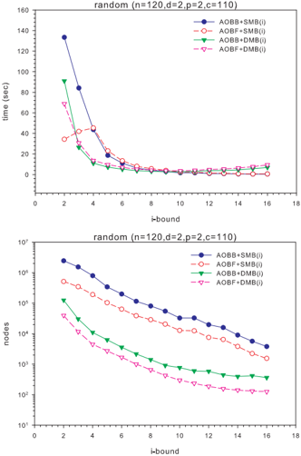
Random Belief Networks We have generated a class of random belief networks using the parametric model ( n, d, c, p ) proposed in [2]. Figure 2 reports the average time results in seconds and number of nodes visited for 20 random instances of a network with n = 120 variables, domain size d = 2 , c = 110 probability tables (CPTs) and p = 2 parents per CPT. The average induced width and pseudo-tree depth were 20 and 32, respectively. The minibucket i -bound ranged between 2 and 16.

When comparing the best-first versus the depth-first algorithms using static mini-bucket heuristics, we observe that AOBF+SMB( i ) is better than AOBB+SMB( i ) only for relatively small i -bounds (i.e., i ∈ { 2 , 3 , 4 } ) which generate relatively weak heuristic estimates. As the i -bound increases and the heuristics become strong enough to cut the search space substantially, the difference between Branch-and-Bound and best-first search decreases, because Branch-and-Bound finds close to optimal solutions fast, and therefore will not explore solutions whose cost is below the optimum, like best-first search.

When looking at the algorithms using dynamic mini-bucket heuristics, we notice that AOBF+DMB( i ) is slightly bet-

1 Available at http://reasoning.cs.ucla.edu/samiam. We used the batchtool 1.5 provided with the package.

ter than AOBB+DMB( i ) only for the smallest reported i -bound, namely i = 2 . This is because these heuristics are more accurate compared to the static ones, and the savings in number of nodes caused by best-first search do not transform into time savings as well. When comparing the static versus dynamic mini-bucket heuristic we observe that the latter is competitive only for relatively small i -bounds (i.e., i ∈ { 2 , 3 , 4 , 5 , 6 } ). At higher levels of the i -bound, the accuracy of the dynamic heuristic does not outweigh its computational overhead. For this reason, in the remaining experiments we only consider the algorithms guided by pre-compiled mini-bucket heuristics.

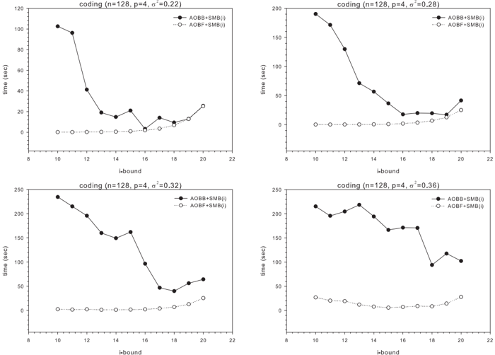
Coding Networks For this domain we experimented with random coding networks from the class of linear block codes . They can be represented as 4-layer belief networks with n nodes in each layer (i.e., the number of input bits). The second and third layers correspond to input information bits and parity check bits respectively. Each parity check bit represents an XOR function of the input bits. The first and last layers correspond to transmitted information and parity check bits respectively. Input information and parity check nodes are binary, while the output nodes are real-valued. Given a number of input bits n , number of parents p for each XOR bit, and channel noise variance σ 2 , a coding network structure is generated by randomly picking parents for each XOR node. Then we simulate an input signal by assuming a uniform random distribution of information bits, compute the corresponding values of the parity

check bits, and generate an assignment to the output nodes by adding Gaussian noise to each information and parity check bit.

Figure 3 displays the average time results in seconds for 20 random coding instances with n = 128 input bits, p = 4 parents for each XOR bit and channel noise variance σ 2 ∈ { 0 . 22 , 0 . 28 , 0 . 32 , 0 . 36 } (we omitted the number of nodes due to space limitations). The average induced width and depth of the pseudo-tree was 54 and 71, respectively. The mini-bucket i -bound varied between 10 and 20. We observe that AOBF+SMB( i ) is far better than AOBB+SMB( i ) for this domain. The difference in CPU time between the best-first and depth-first search approaches is more prominent on the hardest problem instances having higher channel noise variance (i.e., σ 2 ∈ { 0 . 32 , 0 . 36 } ), across all reported i -bounds. SAMIAM was not able to solve any of these problems due to exceeding the memory limit.

Grid Networks In grid networks, the nodes are arranged in an n × n square and each CPT is generated uniformly randomly. We experimented with problem instances developed by [14] for which n ranged between 10 and 38, and 90% of the CPTs were deterministic (i.e., constraints).

Table 1 shows detailed results for experiments with 8 grid networks of increasing difficulty. For each network e nodes were picked randomly and instantiated as evidence. We notice again the superiority of AOBF+SMB( i ) over AOBB+SMB( i ) , especially for relatively weak heuristic estimates which are generated at relatively small i -bounds.

For example, on 90-34-1 , one of the hardest instances, best-first search with the smallest reported i -bound ( i = 12 ) finds the most probable explanation in about 8 minutes (495 seconds) while the depth-first Branch-and-Bound with the same heuristics exceeds the 1 hour time limit. The best performance point on this test instance is achieved for i = 18 , where AOBF+SMB(18) is 9 times faster than AOBB+SMB(18) and explores a search space 23 times smaller. Notice that SAMIAM is able to solve relatively efficiently only the first 3 test instances and runs out of memory on the remaining ones.

Genetic Linkage Analysis The maximum likelihood haplotype problem in genetic linkage analysis is the task of finding a joint haplotype configuration for all members of the pedigree which maximizes the probability of data. It is equivalent to finding the most probable explanation of a belief network which represents the pedigree data [15].

Table 2 displays the results obtained for 12 hard linkage analysis networks 2 . For comparison, we include results obtained with SUPERLINK 1.6. SUPERLINK is currently one the most efficient solvers for genetic linkage analysis, is dedicated to this domain, uses a combination of variable elimination and conditioning, and takes advantage of the determinism in the network.

We observe again that AOBF+SMB( i ) is the best performing algorithm. For instance, on the p42 linkage instance, AOBF+SMB( 14 ) is 18 times faster than AOBB+SMB(14)

2 http://bioinfo.cs.technion.ac.il/superlink/

grid	n	w*		SamIam	AOBB+SMB(i)					AOBF+SMB(i)
	e	h		v. 2.3.2	i=8	i=10	i=12	i=14	i=16	i=8	i=10	i=12	i=14	i=16
90-10-1	100 0	16 26	t #	0.13	0.23 4,396	0.19 3,681	0.08 1,231	0.11 760	0.19 101	0.22 1,788	0.14 1,046	0.08 517	0.09 312	0.19 100
90-14-1	196 0	23 37	t #	11.97	19.95 215,723	12.52 156,387	8.83 112,962	1.22 14,842	0.78 4,209	8.24 46,153	5.97 35,537	2.20 13,990	1.02 5,137	0.70 1,163
90-16-1	256 0	26 42	t #	147.19	1223.55 13,511,366	130.47 1,469,593	11.09 135,746	11.25 123,841	2.38 18,230	133.19 673,238	47.72 250,098	9.91 55,112	10.53 52,644	2.97 11,854
					i=12	i=14	i=16	i=18	i=20	i=12	i=14	i=16	i=18	i=20
90-24-1	576 20	36 61	t #	out	1237.19 6,922,516	285.63 2,051,503	75.02 547,401	22.83 110,144	20.78 15,400	34.21 125,962	38.35 149,445	13.49 49,261	9.08 14,390	21.00 8,155
90-26-1	676 40	35 64	t #	out	-	-	634.59 4,254,454	85.11 455,404	49.97 169,942	out	out	57.66 190,527	29.08 66,429	32.95 24,487
90-30-1	900 60	38 68	t #	out	-	-	365.69 2,837,671	145.86 936,463	37.39 32,637	out	out	40.80 136,576	40.67 121,561	36.00 13,217
90-34-1	1154 80	43 79	t #	out	-	-	974.65 5,555,182	534.10 2,647,012	522.05 2,430,599	494.69 705,922	175.85 303,782	88.24 189,340	59.39 112,955	90.19 115,553
90-38-1	1444 120	47 86	t #	out	-	81.27 259,405	657.91 1,505,849	734.46 1,478,903	133.06 161,156	478.02 580,623	22.80 38,376	47.14 80,177	43.74 52,209	78.05 35,294

Table 1: CPU time in seconds and number of nodes visited for solving grid networks. Time limit 1 hour.

Table 2: CPU time in seconds and number of nodes visited for genetic linkage analysis. Time limit 3 hours.

ped	n	w* h		SamIam v. 2.3.2	Superlink v. 1.6	AOBB+SMB(i)					AOBF+SMB(i)
						i=6	i=8	i=10	i=12	i=14	i=6	i=8	i=10	i=12	i=14
p1	299	15 61	t #	5.44	54.73	4.19 69,751	2.17 33,908	0.39 4,576	0.65 6,306	1.36 4,494	1.30 7,314	2.17 13,784	0.26 1,177	0.87 4,016	1.54 3,119
p38	582	17 59	t #	out	28.36	5946.44 34,828,046	1554.65 8,986,648	2046.95 11,868,672	272.69 1,412,976		out	134.41 348,723	216.94 583,401	103.17 242,429
p50	479	18 58	t #	out	-	4140.29 28,201,843	2493.75 15,729,294	66.66 403,234	52.11 110,302		78.53 204,886	36.03 104,289	12.75 25,507	38.52 5,766
						i=10	i=12	i=14	i=16	i=18	i=10	i=12	i=14	i=16	i=18
p23	310	23 37	t #	out	9146.19	53.70 486,991	49.33 437,688	8.77 85,721	2.73 14,019	3.04 7,089	35.49 185,761	29.29 150,214	10.59 52,710	3.59 11,414	3.48 5,790
p37	1032	21 61	t #	out	64.17	39.16 222,747	488.34 4,925,737	301.78 2,798,044	67.83 82,239		29.16 72,868	38.41 102,011	95.27 223,398	62.97 12,296
						i=12	i=14	i=16	i=18	i=20	i=12	i=14	i=16	i=18	i=20
p18	1184	21 119	t #	157.05	139.06	-	406.88 3,567,729	52.91 397,934	23.83 118,869	20.60 2,972	out	127.41 542,156	42.19 171,039	19.85 53,961	19.91 2,027
p20	388	23 42	t #	out	14.72	7243.43 63,530,037	5560.63 46,858,127	37.28 279,804	95.13 554,623		out	out	33.33 144,212	121.91 466,817
p25	994	29 53	t #	out	-	-	-	-	2041.64 6,117,320	693.74 1,925,152	out	out	out	out	198.49 468,723
p30	1016	25 51	t #	out	13095.83	1440.26 11,694,534	597.88 5,580,555	1023.90 10,458,174	151.96 1,179,236	43.83 146,896	186.77 692,870	58.38 253,465	85.53 350,497	49.38 179,790	33.03 37,705
p33	581	26 48	t #	out	-	886.05 8,426,659	370.41 4,032,864	26.31 229,856	33.11 219,047	54.89 83,360	out	194.78 975,617	24.16 102,888	32.55 101,862	58.52 57,593
p39	1272	23 94	t #	out	322.14	-	-	968.03 7,880,928	61.20 313,496	93.19 83,714	out	out	68.52 218,925	41.69 79,356	87.63 14,479
p42	448	25 76	t #	out	561.31	-	-	2364.67 22,595,247			out	out	133.19 93,831

Table 3: CPU time in seconds and number of nodes visited for solving UAI'06. Time limit 30 minutes.

bn	n	w*		SamIam v. 2.3.2	AOBB+SMB(i)					AOBF+SMB(i)
		h			i=16	i=18	i=20	i=21	i=22	i=16	i=18	i=20	i=21	i=22
BN 031	1153	46 160	t #	out	1183.49 3,990,212	541.82 2,131,977	217.80 889,782	83.08 94,507	145.55 97,721	187.95 427,788	125.94 292,293	83.89 114,046	71.53 25,392	132.55 30,067
BN 033	1441	43 163	t #	-	1717.53 2,156,432	157.17 210,552	190.77 256,191	129.74 89,308	154.16 46,312	80.58 124,453	41.25 41,865	73.70 49,760	94.52 22,256	143.58 14,894
BN 035	1441	41 168	t #	-	67.74 174,370	133.28 243,533	58.81 65,657	80.64 58,973	157.83 45,758	27.25 31,460	36.75 34,987	51.20 15,953	75.53 18,048	158.17 18,461
BN 037	1441	45 169	t #	-	34.77 69,326	21.28 33,475	45.20 8,815	90.35 16,400	144.60 12,507	12.80 16,304	19.25 11,046	45.88 4,315	90.30 5,610	146.61 4,798
BN 039	1441	48 162	t #	-	-	1727.89 3,448,072	475.26 1,043,378	246.60 518,011	653.83 3,045,139	out	254.25 725,738	113.97 213,676	112.69 127,872	211.84 239,838
BN 041	1441	49 164	t #	-	257.96 354,822	56.66 77,653	54.36 38,467	78.74 31,763	130.94 38,088	36.22 94,220	22.20 20,485	43.56 16,549	69.91 11,648	121.24 16,533
BN 127	512	57 74	t #	out	1798.57 17,583,748	-	-	128.55 860,026	113.06 93,543	54.03 235,416	58.84 251,134	64.53 166,741	66.34 84,007	121.53 70,351
BN 129	512	52 68	t #	out	640.29 6,150,175	-	1439.32 13,437,762	222.17 1,747,613	155.63 671,931	out	200.47 922,831	135.60 537,371	out	231.95 622,449
BN 131	512	48 72	t #	out	-	43.06 396,234	51.16 303,818	-	156.11 759,649	19.67 82,780	50.58 209,748	36.66 73,163	65.75 120,153	99.20 46,662
BN 134	512	52 70	t #	out	-	-	-	-	234.38 1,438,986	out	86.80 373,081	96.21 377,064	97.28 214,591	112.63 102,530

and explores a search space 240 times smaller. On some instances (e.g., p1 , p23 , p30 ) the best-first search algorithm AOBF+SMB( i ) is several orders of magnitude faster than SUPERLINK. The performance of SAMIAM was very poor on this dataset and it was able to solve only 2 instances.

UAI'06 Evaluation Dataset We also experimented with 10 belief networks from the UAI'06 Evaluation Dataset 3 . We were not able to obtain the code from the other competitors ( i.e. , Teams 1 and 2) in the MPE evaluation, and therefore we only compare against AOBB and SAMIAM.

Table 3 displays a summary of the results. We observe that AOBF+SMB( i ) is the best performing algorithm on this dataset. While on the first 6 instances AOBF+SMB( i ) improves only slightly causing on average a 2.5 speed-up over AOBB+SMB( i ) , on the remaining 4 instances, the difference between best-first and depth-first search is more dramatic. For example, AOBF+SMB(18) solves the BN 134 instance in less than 2 minutes, while AOBB+SMB(18) exceeds the 30 minute time limit. We notice that in some cases (e.g. BN 127 , BN 129 ), especially for large minibucket i -bounds (e.g. i = 22 ) which generate very accurate heuristic estimates, the savings in number of nodes caused by AOBF+SMB( i ) do not outweigh its overhead.

Summary of experiments. In summary, best-first AND/OR search with static/dynamic mini-bucket heuristics improves dramatically over depth-first AND/OR Branch-and-Bound search, especially for relatively weak heuristic estimates which are generated for relatively small mini-bucket i -bounds. This is significant because it allows the best-first search algorithms to push the landmark of computation further as the induced width of the problems increases.

5 CONCLUSION

In this paper we evaluated a best-first AND/OR search algorithm which extends the classic AO ∗ algorithm and traverses a context-minimal AND/OR search graph for solving the MPE task in belief networks. The algorithm is guided by mini-bucket heuristics which can be either pre-compiled or assembled dynamically during search. The efficiency of the best-first AND/OR search approach compared to the depth-first AND/OR Branch-and-Bound search is demonstrated empirically on various random and real-world benchmarks, including the very challenging ones that arise in the field of genetic linkage analysis.

Our approach leaves room for further improvements. The space required by AOBF can be enormous, due to the fact that all the nodes generated by the algorithm have to be saved prior to termination. Therefore, AOBF can be extended to incorporate a memory bounding scheme similar to the one suggested in [16].

3 http://ssli.ee.washington.edu/bilmes/uai06InferenceEvaluation

Acknowledgments

This work was supported by the NSF grant IIS-0412854.

References

1. J. Pearl. Probabilistic Reasoning in Intelligent Systems. Morgan-Kaufmann, 1988.
2. K. Kask and R. Dechter. A general scheme for automatic generation of search heuristics from specification dependencies. Artificial Intelligence , 2001.
3. R. Marinescu and R. Dechter. And/or branch-andbound for graphical models. In IJCAI , pages 224229, 2005.
4. R. Dechter and R. Mateescu. And/or search spaces for graphical models. Artificial Intelligence , 2006.
5. R. Marinescu and R. Dechter. Memory intensive branch-and-bound search for graphical models. In AAAI , 2006.
6. R. Marinescu and R. Dechter. Best-first and/or search for 0-1 integer programming. In CPAIOR , 2007.
7. R. Marinescu and R. Dechter. And/or branch-andbound search for pure 0/1 integer linear programming problems. In CPAIOR , pages 152-166, 2006.
8. R. Marinescu and R. Dechter. Best-first and/or search for graphical models. In AAAI , 2007.
9. E. Freuder and M. Quinn. Taking advantage of stable sets of variables in constraint satisfaction problems. In IJCAI , pages 1076-1078, 1985.
10. R. Dechter and J. Pearl. Generalized best-first search strategies and the optimality of a*. In Journal of ACM , 32(3):505-536, 1985.
11. Nils J. Nilsson. Principles of Artificial Intelligence. Tioga, 1980.
12. R. Dechter and I. Rish. Mini-buckets: A general scheme for approximating inference. ACM , 2003.
13. A. Darwiche. Recursive conditioning. Artificial Intelligence , 126(1-2):5-41, 2001.
14. T. Sang, P. Beame, and H. Kautz. Solving Bayesian networks by weighted model counting. In AAAI , pages 475-482, 2005.
15. M. Fishelson, N. Dovgolevsky, and D. Geiger. Maximum likelihood haplotyping for general pedigrees. Human Heredity , 2005.
16. P. Chakrabati, S. Ghose, A. Acharya, and S. de Sarkar. Heuristic search in restricted memory. In Artificial Intelligence , 3(41):197-221, 1989.