Causal Discovery from Changes

Jin Tian and Judea Pearl Cognitive Systems Laboratory Computer Science Department University of California, Los Angeles, CA 90024 {jtian, judea } @cs. ucla.edu

Abstract

We propose a new method of discovering causal structures, based on the detection of local, spontaneous changes in the un­ derlying data-generating model. We ana­ lyze the classes of structures that are equiv­ alent relative to a stream of distributions produced by local changes, and devise algo­ rithms that output graphical representations of these equivalence classes. We present ex­ perimental results, using simulated data, and examine the errors associated with detection of changes and recovery of structures.

1 Introduction

In recent years, several graph-based algorithms have been developed for the purpose of inferring causal structures from empirical data. Some are based on detecting patterns of conditional inde­ pendence relationships [Pearl and Verma, 1991, Spirtes et al., 1993], and some are based on Bayesian approaches [Cooper and Herskovits, 1992, Heckerman et al., 1 99 5 ] . These discovery methods assume static environment, that is, a time-invariant distribution and a time-invariant data-generating model, and attempt to infer structures that encode dynamic aspects of the environment, for example, how probabilities would change as a result of interventions. This transition, from static to dynamic information, constitutes a major inferential leap, and is severely limited by the inherent indistinguishability (or equivalence) relation that governs Bayesian networks [Verma and Pearl, 1990].

One way of overcoming this basic limitation is to augment the data with partial causal knowledge, if such is available. [Spirtes et al., 1993], for exam­ ple, discussed the use of experimental data to iden­ tify causal relationships. [Cooper and Yoo, 1999] dis- cussed a Bayesian method of causal discovery from a mixture of observational and experimental data.

We propose a new method of discovering causal rela­ tions in data, based on the detection and interpreta­ tion of local spontaneous changes in the environment. While previous methods assume that data are gener­ ated by a static statistical distribution, our proposal aims at exploiting dynamic changes in that distribu­ tion. Such changes are always present in any realistic domain that is embedded in a larger background of dynamically changing conditions. For example, nat­ ural disasters, armed conflicts, epidemics, labor dis­ putes, and even mundane decisions by other agents, are unexpected eventualities that are not naturally captured in distribution functions. The occurrence of such eventualities tend to alter the distribution un­ der study and yield changes that are markedly dif­ ferent from ordinary statistical fluctuations. Whereas static analysis views these changes as nuisance, and attempts to adjust and compensate for them, we will view them as a valuable source of information about the data-generating process. A controlled experimen­ tal study may be thought of as a special case of these environmental changes, where the external influence involves fixing a designated variable to some predeter­ mined value. In general, however, the external influ­ ence may be milder, merely changing the conditional probability of a variable, given its causes. Moreover, in marked contrast to controlled experiments, we may not know in advance the nature of the change, its lo­ cation, or even whether it took place; these may need to be inferred from the data itself.

The basic idea has its roots in the economic literature. The economist Kevin Hoover (1990) attempted to in­ fer the direction of causal influences among economic variables (e.g., employment and money supply) by ob­ serving the changes that sudden modifications in the economy (e.g., tax reform, labor dispute) induced in the statistics of these variables. Hoover assumed that the conditional probability of an effect given its causes

remains invariant to changes in the mechanism that generates the cause, while the conditional probability of a cause given the effect would not remain invariant under such ch an g es . This asymmetry may be useful in dis t in g u i s hi n g cause and effect.

Today we understand more precisely the conditions under which such asymmetries would prevail and how to interpret such asy m me t r ies in the context of large, multi-variate systems. Whenever we obtain reliable in­ formation (e.g., from historical or institutional knowl­ edge) that an abrupt l o c al c h a n ge has taken place in a specific mechanism that constrains a given fam­ ily of variables, we can use the observed changes in the ma r g i n a l and conditional probabilities surround­ ing those variables to determine the direction of causal influences in the domain. The statistical features that remain invariant under such changes, as well as the causal assumptions underlying this invariance, are en­ coded in the causal diagram at hand, and can be used therefore for testing the validity of a given struc­ ture. L ik ew is e , conflicts between observed and pre­ d icte d changes can be used for automatic r est ruc t u r ing of the topology of the structure at hand.

2 Causal Models and Mechanism Change

Let our problem domain be a s et of discrete ran­ dom variables V = {V1, .. . , Vn}· We assume that a causal model over V is a pair M = <G, 8a>, where G is a DAG over V, called a causal diagram, and 8a is a set of probability parameters. We as­ sume that each variable Vi can take values from a finite domain, Dm(Vi) ={vi!,··· ,Vir.}, where r; is the number of states of V;. We use Pai to repre­ sent the s et of parents of Vi in a causal diagram G and Dm(Pai) to r e pr es e nt the set of states of Pa;. Let Bv,;pa., v; E Dm(V;),pa; E Dm(Pa;) denote the multinomial parameter corresponding to the condi­ tional probability P(v;lpai)· We will use the follow­ ing notations: �a, = {Bv;;pa; !vi E Dm(Vi)}, lli ; = Upa;EDm(Pa;) e;, a,, 8a ur=l V;. Assuming the Causal Markov condition [Spirtes et al., 1993], a causal model M = <G, 8a> generates a probability d i s t r ibu ti on

A probability distribution P(V) is said to be compati­ ble with a causal diagram G i f P(V) can be generated by some causal model M == <G, 8a>.

The factorization in Eq. (1) obtains causal character through the assumption of modularity; each family in the causal diagram represents an autonomous physical mechanism and is subjected to change without influ­ encing other mechanisms. We f o r m all y define mecha­ nism change as follows.

Definition 1 (Mechanism Change) A mechanism change to a causal model M = <G, 8a> at a variable Vi is a transformation of M that produces a new model, Mv, = <G, 8(;,>, where 8(;, ='II� U (8a \ ii";) and ii� is a set of parameters having values that differ from those in 1li;.

We assume in this paper that the parent set Pa; does not change in a mechanism change. An intervention that fixes v; to a particular value is a special case of a mechanism change. Let P(V) be the distribution generated by M, as in Eq. (1). Then the distribution generated by Mv, is given by

We will call (P, Pv,) a transition pair (TP) and Vi t he focal variable of the transition. Assume that a series of mechanism changes occurred successively to a causal model M = <G, 8�>, and l et F = (Vi1, · · · , Vi�) de­ note the corresponding sequence of focal variables. We use Pr 8 = ( P0, Pl, .. . , pk) to denote the sequence of distributions generated by such a series, and call the pair (Prs, F) a transition sequence (TS).

As oracles for cause-and-effect relations, causal mod­ els can predict the effects t h a t any external or sponta­ neous changes have on the distributions. Conversely, by detecting how probability distributions change un­ der various mechanism changes, we obtain information on the structure of the model generating those distri­ butions. In this paper, we assume t h at we are given a TS (Prs, F) corresponding to some causal diagram G, and our task is to recover G. We will then assume that we have a sequence of datasets IIJ.I.rs = {D0, . . · , D k }, where each Di is a set o f random samples from a dis­ tribution pi, such that each pair (Pi-1, Pi) is a TP with focal variable v;i, and our task will be to recover a causal diagram (or a set of diagrams) that can gen­ erate li}ys. First, we study what can be learned from a TS.

3 Indistinguishability of Causal Diagrams

In this section, we study the classes of causal structures that are indistinguishable (or "equivalent") relative to a TS.

The statistical information provided by any causal di­ agram is completely encoded in the independence rela­ tionships among the variables. Therefore, two causal

diagrams are statistically indistinguishable given one static distribution if and only if they are independence equivalent. The graphical conditions for independence equivalence are given by the following theorem.

Theorem 1 (Independence Equivalence) Two causal diagrams are independence equivalent if and only if they have the same skeletons and the same sets o f v-structures, that is, two converging arrows whose tails are not connected by an arrow (Verma and Pearl 1990).

Now assume that we have a TP with focal variable V;. A causal diagram G is said to be compatible with a transition pair (P, Pv,) if P can be generated by a causal model M = <G, 0a> and Pv, can be gen­ erated by a causal model Mv. = <G, 00> resulted from a mechanism change to M at V;;. Note that a causal diagram could be compatible with both P and Pv, but not compatible with the TP (P, Pv;). Among those independence-equivalent diagrams com­ patible with both P and Pv., a TP (P, Pv,) can dis­ tinguish those that can generate Pv, from P with a single mechanism change from those that can not. Two causal diagrams G1 and G2 are called transi­ tion pair equivalent with respect to a TP with focal variable V;, or Vi-transition equivalent, if every TP (P, Pv,) compatible with G1 is also compatible with G2. Two causal diagrams are statistically indistin­ guishable given a TP (P, Pv.) if and only if they are Vi-transition equivalent.

Theorem 2 (Transition Pair Equivalence) Two causal diagrams G1 and G2 are V; -transition equiva­ lent if and only if they have the same skeletons, the same sets of v-structures, and the same sets of parents for V;;.

Proof" Let G1 be compatible with a TP (P, Pv.). G2 must have the same skeletons and the same sets of v­ structures as G1 to be compatible with P (and Pv.) by Theorem 1. We have the following decomposition:

where Pa: and Paf are parents of V; in G1 and G2 respectively. G1 is compatible with the TP (P, Pv.), hence can generate Pv. from P by a mechanism change at Vi:

Plugging the expression for f1#i P(vilpa}) Eq. (3) into Eq. (4), we have from

A

G2 is also compatible with the transition pair (P, Pv.) if and only if

Eqs. (5) and (6) lead to

.

which holds for any distribution P and Pv. if and only if G1 has the same parent set for Vi as G2 (Pa} = Pat); if G1 has a different parent set for Vi with G2, Eq. (7) will impose some constraints between P and Pv,, and will not hold for arbitrary possible transition pair ( P, Pv. ) . D

A TS is simply a series of TP's. Accordingly, we say that a causal diagram is compatible with a transition sequence Prs = (P0, P1, .. . , pk), F = (Vi., . . . , Vi�o) if it is compatible with each TP (Pi-l, Pi) in the se­ quence. Likewise, two causal diagrams G1 and G2 are called transition sequence equivalent with respect t o a TS (Prs, F), or F-transition equivalent, if every TS (Prs,F) compatible with G1 is also compatible with G2. Two causal diagrams are statistically indistin­ guishable given a TS (Prs, F) if and only if they are F-transition equivalent.

Theorem 3 (Transition Sequence Equivalence) Two causal diagrams are F -transition equivalent if and only if they have the same skeletons, the same sets of v-structures, and the same sets of parents for variables in F.

Theorem 3 says that a TS determines the directions of the edges between the focal variables and their neigh­ bors (among the set of independence-equivalent dia­ grams). Figure 1 shows an example ofTS equivalence. Given a TS, the most we can expect to recover is a set of causal diagrams that are TS-equivalent, as defined by Theorem 3. We may find this equivalence class by detecting independence relations and distribution changes.

4 Learning Causation by Detecting Changes

In this section, we identify the causal information that can be learned by detecting various changes in the probability distributions, in particular, changes in the marginal probability of each variable. The following theorem is obvious.

Theorem 4 A mechanism change at a variable X to a causal model M = <G, So> may alter the marginal probabilities of the descendants of X in G and can not alter the marginals of nondescendants of X.

It is possible of course that, for some peculiar parame­ ter changes, the marginal probabilities of some descen­ dants of X would not change. When recovering causal information from distributional changes, we assume a restriction on a TS called influentiality.

Definition 2 (infiuentiality) A TP (P, Px) gener­ ated by a causal model <G, 0a> is said to be influen­ tial if for every descendant Y of X in G, the marginal distribution Px (Y) is different from P(Y). A TS is influential if every TP in the sequence is influential.

Given a TP (P, Px ) , and assuming that we can test each variable for marginal distribution change, we can draw the following inferences. If the marginal of a variable Y has changed, we conclude that Y is a de­ scendant of X. If the marginal of a variable Z has not changed, we conclude that Z is a nondescendant of X. We thus conclude that Z < X < Y should be a causal order consistent with the causal diagram. Next we discuss how to piece together ordering information of this kind, as obtained from a TS.

4.1 Partitioning the variables

Given a TS PTS, F = (Viu . .. , Vi.), each variable can be characterized by a sequence of 1's and O's, a tag a1, ... , a,_, where a1 reflects whether the marginal of that variable changed ( a; = 1) or not ( ai = 0) in the ith transition of the sequence. Non-focal variables that are given the same tags cannot be distinguished by the TS (through detecting marginal changes), and no in­ formation can therefore be extracted about their rela- tive causal order in the causal diagram. We may put all such variables into a bucket labeled w i t h the same tag, denoted by B a 1··· a � . Clearly, since we have no in­ formation on causal relations among variables within the same bucket, all variables in a bucket stand in the same ordering relation to all variables in another bucket. Focal variables need special treatment since they carry more information, and we will put each fo­ cal variable into an individual bucket called a focal bucket, denoted by B[1 . . · a� .

We classify variables into buckets with the following algorithm.

Algorithm 1 (Partitioning Variable)

Input: a TS PTs, F = (Vi1, · · · , Vi�o )·

Output: A set of buckets, each associated with a tag a1 . . . a,., and each containing a set of variables.

Put all variables in a bucket B.

For each bucket Ba1···a;_1 including focal buckets if it contains the i th focal variable, put it in a focal bucket B ! 1 ... a,_11.

For the ith mechanism change, i = 1, ... , k, put other changing variables in Ba1···a,_1 1· put non-changing variables in Ba1 . . · a,_1o.

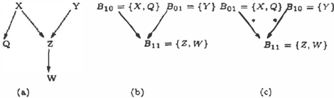
We show the partitioning process by an example. As­ sume that the actual causal diagram is the DAG shown in Figure 2(a) and that we are given a TS (P, Px, Py ) . In the first transition, with X as the fo­ cal variable, P(Y) does not change, hence B0 = {Y}; P(X),P(Z),P(W),P(Q) do change, hence we form B 1 = {Z, W, Q}, B{ = { X }. Note that a focal vari­ able is put into an individual bucket. In the second transition, withY as the focal variable, P(Y) changes, giving B £ 1 = {Y}; P(Z) and P(W) change, giving B11 = {Z, W}; P(Q) and P ( X ) do not change, giving Bw = {Q} and B{0 ={X}. As a result, the variables are partitioned into four buckets: B{0 = {X}, B6 1 = {Y},B10 = {Q}, Bn = {Z, W}.

4.2 Extracting causal information

We shall now discuss what causal information we can extract from the tags attached to buckets. Consider any two buckets Ba1 ... 0�< and Bb1 . . . h. If there exists a bit such as ai < b i (i.e., ai = 0 and bi = 1), it must be that, in the ith transition, the marginals of variables in Ba1 ... a� did not change and the marginals of variables in Bb1 ... b� did. Therefore, no variable in Ba1 ... 0� is a descendant of any variable in Bb1 · · · b h . On the other hand, if there exists another bit such that aj > bi (a j = 1, bj = 0), then no variable in Bh .. ·b�. is a descendant of any variable in Ba1 . . . ak, which means that there exists no directed path, in particular no edge, between any variable in Ba1 . . · ak and any vari-

able in Bb t .. · b �< . The equality a; = b;, i = 1, . .. , k can only happen if one of the buckets is a focal bucket, in which case the focal variable is an ancestor of all the variables in the other bucket. In summary, the relation between two buckets B a t .. -a., and Bb1 ... b., is determined as follows:

• R1 a; � b;, i = 1, ... , k and 3j, ai < b1: variables in Ba1 ... a�< are nondescendants of variables in Bb1 . .. b �< , denoted by B at"·a· < Bh . . · h ·
• R2 a;;::: b;,i = 1, ... ,k and 3j,ai > b1: Bb1· .. b n < Bat·"ak ·
• R3 There exist two bits i =/: j such that a; < b; and a1 > b1: there can be no directed path be­ tween any variable in Bat .. -a · and any variable in B&, .. -b., ·
• R4 a; = b;, i = 1, .. . , k, one of the buckets, say B t . . a�<, is a focal bucket: all variables in Bb, ... h must be descendants of the focal variable in B £ 1 .. -a�<, which is a stronger relation than that in R1 and R2 but will still be denoted by B [ t . .. a., < Bb, .. ·b··

The focal buckets convey more information. Let Bat .. ·a· be a focal bucket containing the focal vari­ able Vi; for the jth transition. Then if bi = 1, we have that all variables in B & , ... b�< are descendants of v;, since their marginals changed in the jth transi­ tion. This rule is consistent with the above rules R1R3, hence it is applied only in R4 when R1-R3 cannot determine a relation. However, in practice, due to im­ perfect statistical tests, there may be conflicts between them. For example, we may determine that there is no edge between Bat ... a�< and Bbt . .. h by R3 and in the same time Ba1 .. . a . is a focal bucket for the jth transi­ tion and bj = 1. These conflicts signal mistakes in the statistical tests, and whenever there are conflicts, we will declare the relation as "unknown". We summarize the above discussions with the following algorithm.

Algorithm 2 (Extracting Relation)

Input: two buckets Ba1 ... ak and Bb 1 . .. h. "

Output: the relation between the two buckets, could be "< , "no-directed-path (NDP) ", or "unknown".

1. a;� b;,i = 1, ... ,k and 3j,ai < b1: ifBb1 . . . b�< is a focal bucket for the lth transition and ac = 1 then "unknown", else Ba1 .. · a· < Bbt ... b., .
2. a; ;::: b;, i = 1, .. . , k and 3j, ai > bi: if B(w . . a�< is a focal bucket for the lth transition and bt = 1 then "unknown", else Bb1 . . . h < Ba1 .. . a ·.
3. There exist two bits i -:j:. j such that a; < b; and ai > bj: if Bb 1 ... b, is a focal bucket for the lth
4. transition and ac = 1 or Ba1 . . . a, is a focal bucket for the lth transition and b1 = 1 then "unknown", else "NDP".
5. 4a; = b;, i = 1, .. . , k: if both buckets are focal buckets then "unknown", else let the focal bucket be st . . . . a., then B t 1 ... a�< < Bbt . . . h.

Consider the binary relation "<" on the set of buckets as defined in the Algorithm 2. We have the following theorem.

Theorem 5 The binary relation "< " on the set of buckets is a partial order.

Proof: The relation is transitive. If B a 1 ... a. < Bb1 . . . b . and B&1 . .. & . < Bc1-. . c�<, we have a; � b; � c;, i = 1, ... ,k.

1. 3j, ai < Cj. If Bc1 ... c. is not a focal bucket, then we have Ba1 ... a. < Bc1 ... c.. If Bct ... ck is a focal bucket for the lth transition and az = 1, then bz = 1 since az � b1 � c1, which contradicts Bbt .. . b. < BCt"'Ck'
2. a; = c;, i = 1, ... , k. Then a; = b; = c;, i = 1, ... , k, and then Ba1 ... a. has to be a focal bucket and Bbt ... b, is not one in order to have the re­ lation Bat . . · a · < Bb1 ... & ., which then contradicts Bbt .. ·h < Bct·"Ck·

The relation is antisymmetric. If Ba1 ... a. < Bbt ... h and Bb1 . .. h < B a 1 ... a., then a; = b;, i = 1, ... , k. Since they cannot both be focal buckets, they must be the same bucket. D

A partially ordered set can be represented by a DAG. We construct a graph with both directed and undi­ rected edges, called an order graph ( OG ) , as follows: a node represents a bucket; for each pair of buckets B and B', there is a directed edge B � B' if B < B1; there is an undirected edge B-B' if the relation be­ tween them is "unknown". If we had a perfect statis­ tical test for distributional changes, an OG would be a DAG. For the causal diagram shown in Figure 2(a) and the TS (P, Px, Py), the ideal OG is given in Fig­ ure 2(b).

In an OG, when B is a focal bucket, a directed edge B ---t B' asserts that there exists a directed path from the focal variable contained in B to all the variables in B'. Hence, if there is no other mixed directed path, a path that could contain undirected edges but no di­ rected edges in the reverse direction, from B to B1 in the OG, there must be an edge from B to at least one variable in B' in the causal diagram. We mark this type of edges as B � B1, to distinguish them

二

一

from those that only represent potential edges in the causal diagram. This information is useful when the child bucket B' contains only one variable; we then assert that the edge B � B' must exist in the causal diagram. We will call an OG with marked edges a marked order graph (MOG); an example is shown in Figure 2(c).

An algorithm for constructing a MOG is given in the following.

Algorithm 3 (Constructing MOG)

Input: an influential TS with known focal variables. Output: a marked order graph.

1. Put variables into buckets using Algorithm 1.
2. Extracting relations among buckets using Algo­ rithm 2.
3. Let each bucket be a node.
4. ..{.. For each pair of nodes B and B' If B < B', add an edge B � B'. If B' < B, add an edge B' ---+ B. If the relation is "unknown", add an edge B- B'.
5. For each focal bucket Bf and each of its child B If there is no other mixed directed path from Bf to B, mark the edge as Bf �B.

In summary, the information conveyed by a MOG is as follows:

1. An unmarked edge B � B': All variables in B can be ordered before all variables in B' in the causal diagram, in other words, there are no di­ rected paths from variables in B1 to variables in B. When B is a focal variable, there exists a di­ rected path from B to each variable in B' in the causal diagram.
2. A marked edge B � B': There exists a directed path from B to each variable in B'. In the case that both B and B' contain one single variable, the edge B ---+ B' must exist in the causal dia­ gram.
3. No edge between B and B': there is no directed path, in particular no edge, between any variable in B and any variable in B' in the causal diagram.

4.3 Limitation of detecting marginal changes

Can we fully recover a causal diagram by detecting marginal distribution changes alone? To fully recover a causal diagram, we must construct a MOG in which each bucket contains only one variable and every edge is marked. This may not, in general, be achieved. Considering a causal diagram G containing a path X ---+ Z ---+ Y, it is clear that we can never de­ termine if there is an edge X ---+ Y in G, since all marginal changes produced by transitions would be the same after adding that edge. What is the best we can get then by detecting marginal changes?

Given a DAG G, if we remove an edge X --t Y when­ ever there is a directed path from X to Y, we get the transitive reduction of G. The transitive reduction of a DAG G is the graph G' with the fewest edges such that the transitive closure of G' is equal to the transi­ tive closure of G. The transitive closure of a DAG G is the graph G11 such that an edge X --t Y is in G11 iff there is a directed path from X toY in G. By detect­ ing marginal changes in TS's, the best we can hope to get is the transitive reduction of the actual causal diagram. Since to mark an edge X ---+ Y, X must be a focal variable, it follows that every node except leaf nodes must be a focal variable in order to mark ev­ ery edge in the transitive reduction graph. To further make each bucket contain only one variable, every leaf node having the same set of parents as another leaf node must be a focal variable.

In conclusion, by detecting marginal distribution changes, the best we can learn is the transitive reduc­ tion of the causal diagram, and we can achieve it by a TS in which every variable has had its mechanism changed.

4.4 Unknown focal variables

In this section we discuss si�uations where we know that a mechanism change has occurred at a single vari­ able but we do not know the identity of that variable.

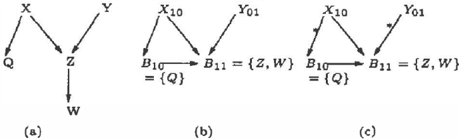
We first note that, without knowing the focal vari­ ables, variables can still be partitioned into buckets using Algorithm 1, and the relations between pairs of buckets will be determined by rules Rl-R3 of Sec­ tion 4.2. Second, an order graph can be constructed as follows: for each pair of buckets B and B', there is a directed edge B ---+ B' if B < B'. For the causal diagram of Figure 3(a) and the TS (P,Px,Py), the variables are partitioned into three buckets: B10 = {X,Q},Bol = {Y},Bu = {Z, W}, and the OG is

Figure 3: (a) A causal diagram; (b) The order graph for the TS ( P, Px, Py) without knowing the focal vari­ ables; (c) The marked order graph.

shown in Figure J(b).

Finally, we may be able to find to which bucket a focal variable belongs using the following theorem, assuming influentiality and perfect statistical tests. (We still call such a bucket a "focal bucket", because it behaves as a focal variable with the information at hand.)

Theorem 6 Let Si be the set of buckets f or which a i = 1 in their tags a1 . . . a k , then the f ocal bucket p i for the jth transition is in Sj and for any other bucket BE S i , p i < B.

Proof: Let the focal variable X for the jth transition be tagged as a1 . . · ak, then ai == 1, since P(X) must change in this transition. All other variables in the set of buckets Si must be descendants of X since all their marginals changed in the jth tran­ sition. Therefore, whenever P(X) changes, their marginals must change too, that is, if ai = 1 then bi = 1 f o r any variable tagged as b1 ... bk in Sj, which leads to ai � b;, i == 1, ... , k. Hence for any bucket Bbt . . . b& E S i not containing X, we have Ba1 · . . a� < Bb, . .. bk· D

In practice, Theorem 6 may fail to identify a focal bucket when (due to imperfect statistical tests) there exists no bucket p i in Sj satisfying p i < B for any other bucket B E Si. In the case that an identified focal bucket contains only one variable, we actually identify a focal variable. For the OG in Figure 3(b), the focal buckets for the first and second t r an s itio n s can be found as B 1 0 = {X, Q} and B01 = {Y} respec­ tively, and we actually identify Y as the focal variable of the second transition.

Finally we can get a MOG by marking edges as in Algorithm 3. For our working example, the ideal MOG is shown in Figure 3(c).

4.5 TSs absent of influentiality

If we allow for the possibility that a mechanism change at X may not alter the marginal probabilities of some of X's descendants, t he n detecting no change in P(Y)

provides no information on the causal relation between X and Y. The information we may obtain is that de­ tecting a change in P(Y) means that Y is a descendant of the focal variable X. First we partition variables into tagged buckets using Algorithm 1. Then the re­ lationship among buckets is determined as: l et B i be the focal bucket for the ith transition; Bi < Ba1 ... a � if ai = 1, where "<" represents that all variables in Ba1 ··· Cik are descendants of the focal variable B ' . Fi­ nally we compute the transitive closure of <: relation, denoted by <*, to get more information. Simultane­ ous B <* B' and B' <* B would mean change detec­ tion errors and the relation between B and B' will be declared as unknown. The information conveyed by B <· B' is that all variables in B' are descendants of the focal variable B in the underlying causal diagram.

It is clear that if the identities of the focal variables are not given, we can not get any order information from a TS by detecting marginal changes.

5 Combining Static and Dynamic Information

In Section 4, we discussed how to extract causal infor­ mation given a TS by detecting distributional changes. In this section, we briefly describe h ow to c o m b i n e this information with that obtained from independence tests.

Given data from a static stable distribution, we can re c o v e r (partially directed) causal diagrams us­ ing conditional independence tests. Several such algorithms have been developed, including IC al­ gorithm [Pearl, 2000, section 2.5] (initially intro­ duced in [Pearl and Verma, 1991]) and PC algo­ rithm ( S pi r t es et al., 1993]. The outp u t of th e se algo­ rithms is a partially oriented graph representing an independence-equivalence class as defined by Theo­ rem 1.

To recover a causal diagram from a TS, we first extract causal information by detecting distribution changes as d es c ri b e d in Section 4, then run the IC algorithm using the causal information as prior knowledge. Note that since a TS is composed of a series of different dis­ tributions, we need to test independence relationships across all distributions.

We may obtain three types of causal information as shown in S e c t io n 4: causal order among certain vari­ ables, no edges between certain variables, and cer­ tain directed edges. The last two types (no-edge and determined-edge) can be incorporated directly. Causal order information can be used to restrict the search of candidate conditional sets and thus reduce the com­ plexity of the IC algorithm. Causal order information

can also be used to orient more edges: any undirected edge X-Y can be oriented as X --+ Y if X is ahead of Y in the causal order. These methods of incorpo­ rating background knowledge have been discussed in [Spirtes et al., 1993, Section 5.4.5].

When the identities of all focal variables are known, after incorporating these causal information as back­ ground knowledge, the output of the IC Algorithm would be a partially oriented graph representing the TS equivalence class as defined by Theorem 3. This is due to a theorem in [Meek, 1995] which says that the orientation rules in the IC algorithm are complete with respect to any consistent background knowledge. If the identity of a focal variable is not given or iden­ tified as in Section 4.4, the edge directions between this focal variable and its neighbors may not be fixed, hence the output graph is not maximally oriented, and we have not obtained all the information implied by a TS. Algorithms for identifying focal variables are cur­ rently under investigation.

6 The Bayesian Approach

In the Bayesian approach, we compute the posterior probability of a causal diagram G given a dataset D as:

where t;, represents our background knowledge. For the case that the dataset D is from a static dis� tribution, closed form expressions for P(DIG, ) have been derived [Cooper and Herskovits, 1992, Beckerman et al., 1995]. In this section, we gave a closed form expression for P(s IG,t;,). For detailed derivation, see [Tian and Pearl, 2001].

Let the sequence of datasets llll-rs = {D0 ,Dt, ... , Dk} be generated With parameters e�l . .. I e2. respec­ tively, and let 3a = Uf=o e h . The marginal likelihood is computed as

We have put F = (Vi1 , � � � , Vi) as a condition to re� flect the fact that the sequence of focal variables are known. The term P(IThrs l2a1 01 ) is computable as the probability of the data given a Bayesian network. For the parameter priors P(2aiG, F, t;,), we use the assumptions given in (Beckerman et al., 1995]: Global and Local Parameter Independence, and Parameter

Modularity, and we assume the following prior:

where o(x) is the Dirac delta function, and we have used the notation eb = Uf;l w{ I j = 0, . . . ' k. Eq. (10) says that the set of parameters eb d i ff e r s with eb-1 only by the parameters in IP{i, and we have made an assumption that the set of parameters w{. J after a mechanism change is independent of the previous set of parameters �P{i-1. We assume the Dirichlet distribution:

where Opa; = { C:tv; ;pa; lv; E Dm(V.)} denotes the set of parameters for the Dirichlet distribution. As­ suming that the set of parameters after a mecha­ nism chan�e have the s�e prior distribution as be­ fore: P(wf.IG,{) = P(�f-1jG,�), and that mecha-' ' nism changes occurred at different variables, let I = {i1, · . . ,i�;} be the set of indexes for focal variables, and we obtain

where ro is the Gamma function, O:pa; = Ev. O:v;;pa.,

and NLva; is the number of cases in the dataset Di for which V. takes the value V i and its parents Pa; takes the value pai.

We will call the above Bayesian scoring metric P(Drs, GIF, ) with parameters au,;po.; specified as re� quired by the BDe metric in [Beckerman et a.l., 1995]

the BDe_TS metric. A marginal likelihood P(IDl/ G, �) is said to satisfy the property of F -transition likelihood equivalence if for two F-transition equivalent causal di­ agrams G1 and G 2 , P(IDIGt , �) = P(IDl/G 2 , 0-

Theorem 7 The BDe_ TS metric is F -transition like­ lihood equivalent.

7 Experimental Results

We use x2 test to detect distribution changes. Let D1 and D2 be two datasets, consisting of N1 and N2 cases respectively. Let N1z and N2x be the number of cases in D1 and D2 respectively in which a variable X takes t he value x. To test the hypothesis that X has the same distribution in the two datasets, we compute the quantity

which is asymptotically a x2 distribution with rx -1 d e g r ee of freedom, where r:r: is the number of states of X. Let the significance level be o:. I f x2 > x! then we decide "change" , else we decide "no-change" .

A mechanism change at a variable Vi is simulated as follows. Consider parameters in �a; . If 8v,1;pa; ::; 0.5 then let Ov ' . 1 ·pa · = Bv-1 ·pa + o, else let Ov ' . ·pa · = t 1 t \ ' ,. ... . , 1Bvn;pa; -o, where o is a parameter for adjusting the change magnitude. The rest of the parameters in �a, are changed in proportional to their original values as: O�,;;pa, = o:Ov,j;pa. , j = 2, . . . , r;, where o: = (1 0�n;paJ/(1 -0v,1;pa. ). When we simulate a mechanism change at Vi, we change parameters in �a, as above for each pa; E Dm(Pa;).

In our experiments, we used data generated from a known network, t h e Alarm Bayesian network1 [Beinlich et al., 1989]. Samples used in the experiment were generated from the network using a demo version of Netica API developed by Norsys Software Corpo­ ration. We used equal sample sizes for all datasets in a TS, that is, a sample size N represents that N cases were generated for each dataset Di in lilTs = {Do, . . . , D k }.

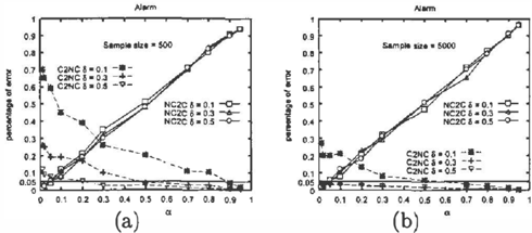
7.1 Errors in detecting changes

There are two types of errors in detecting changes: (i) mistaking "no-change" for a "change", known as type I error and denoted NC2C, and (ii) mistaking "change" as "no-change" , known as type II error and denoted C2NC. Let G be the causal diagram used for gener­ ating samples. When a mechanism change occurs at

1 We used the version downloaded from the web site of Norsys Software Corporation, http:/ j www .norsys.com.

a variable Vi, if our test statistics is perfect, all Vi 's descendants in G should be identified as "change" and Vi's nondescendants as "no-change" . Let Deci be the number of descendants of Vi in G and N D e c i be the number of non descendants of Vi. Let c2nci be the number of descendants of Vi identified as "no-change" by the x 2 test, and let nc2ci be the number of nonde­ scendants of Vi identified as "change" . nc2ci a,nd c2nc; represent the number of type I and type II mistakes made by the x 2 statistics. In any one run, we simulate a mechanism change at each node Vi, i = 1, . . . , n, rel­ ative to the original network, and compute the C2NC error rate as Li c2nc;j L; Deci and the NC2C error rate as Li nc2c;j L; N Dec;. We computed an aver­ age error rate over 5 runs.

We varied the change magnitude o, the sample size, and the significance level o:, and the results are shown in Figure 4. We see that the NC2C (type I) error rate is nearly the same as the o: value for different change magnitudes and sample sizes, as expected. The C2NC (type II) error could be large when the a value is small or the change magnitude is small. This sug­ gests that we should consider using a two-tailed x2 test [Silverstein et al., 2000] to control the C2NC error, es­ pecially when the sample size is not large. In a two­ tailed x 2 test, we use another threshold o:1 > a such that we decide "no-change" only when x2 < X�,, but we have to decide "unknown" when x!, < x 2 < x!­ We will not discuss this method in this paper.

7.2 Errors in order graphs

In an OG, an edge B ---+ B' represents that all vari­ ables in B can be causally ordered before the vari­ ables in B'. We call this type of information "order claims" . No edge between B and B1 represents the absence of directed paths, in particular edges, between variables in B and those in B1; this information will be called "no-directed-path (NDP) claims" and "no­ edge claims" respectively. An edge B-B' only signals mistakes in the statistical tests and will be called "un­ known claims" . We performed the following experi-

Table 1: Errors in order graphs. k: the number of focal variables. m: the number of buckets. Eo: percentage error of order claims. Ep: percentage error of NDP claims. Ee: percentage error of no-edge claims. u: number of unknown claims.

			N = 500
				order claim		NDP claim
k			m	'If	Eo	'If		E.	u
5			8	275	0.13	37		0.049	0
5			1 1	355	0.12	88		0.039	3
5				7		8		7	1
5				391		111		0.03	5
10				354		137		0.044	1
10				335		241		0.044	1 1
10				360				7	5
10				323	0.026	274	0.29	0.032	19
	N = 5000
				order claim		NDP claim
k	&	0:	m	?I	'Eo	?I	Ep	E.
5	0.1	0.01	10	369	0.044	80	0.3	0.025
5	0.1	0.05	12	393	0.051	109	0.3	0.031
5			1					. 1
5	0.5	0.05	12	406		104	0.26	0.027	7
10	0.1	0.01	19	364		207	0.28	0.02	6
10	0.1	0.05	23	334		260	0.28	0.033	20
10	.5	. 1	1	77		1 1
10	0.5	0.05	23	334		265	0.26	0.03	22

ments: for certain 8, a, sample size, and focal vari­ ables, we generate datasets, construct an OG, count the claims, and check against the true network to com­ pute percentage errors for each type of claims.2

The results are shown in Table 1 for various sample size N, number of focal variables k, mechanism change magnitude 8, and significance level a. From Table 1, we see that the NDP claims have a high percentage of error; however, if those claims are interpreted as rep­ resenting no-edge only, then the error rates are much lower. As expected, the error rates are lower when 8, the change magnitude, is larger, and a TS with more focal variables produces more no-edge claims.

8 Conclusion

Spontaneous local changes offer the potential of ex­ tracting causal information that is undetected by static methods. This potential is limited by several factors, the most significant are violation of influential­ ity (in large networks) and the reliance on the locality of the changes. We believe that the former problem

2Claims are counted between pairs of variables not be­ tween pairs of buckets. Numbers vary with the focal vari­ ables picked, hence we did 100 runs, each time randomly picking a sequence of k variables as focal variables, and computed average numbers.

can be overcome by restricting the order information extracted to close neighborhoods of the focal variables.

Acknowledgements

This research was supported in parts by grants from NSF, ONR and AFOSR and by a Microsoft Fellowship to the first author.

References

• [Beinlich et al., 1989] L A. Beinlich, H. J. Suermondt, R. M. Chavez, and Cooper G. F. The ALARM monitoring system. In Proceedings of the second European conference on Artificial Intelligence in Medicine, 1989.
• [Cooper and Herskovits, 1992] G. F. Cooper and E. Herskovits. A Bayesian method for the induc­ tion of probabilistic networks from data. Machine Learning, 9:309-347, 1992.
• [Cooper and Yoo, 1999] G. F. Cooper and C. Yoo. Causal discovery from a mixture of experimental and observational data. In Proceedings UAI, 1999.
• [Beckerman et al., 1995] D. Beckerman, D. Geiger, and D.M. Chickering. Learning Bayesian networks: The combination of knowledge and statistical data. Machine Learning, 20:197-243, 1995.
• [Hoover, 1990] K.D. Hoover. The logic of causal infer­ ence. Economics and Philosophy, 6:207-234, 1990.

[Meek, 1995] C. Meek. Causal inference and causal explanation with background knowledge. In Pro­ ceedings UAI, 1995.

[Pearl and Verma, 1991] J. Pearl and T. Verma. A theory of inferred causation. In Proceedings KR '91.

• [Pearl, 2000] J. Pearl. Causality: Models, Reasoning, and Inference. Cambridge University Press, NY, 2000.
• [Silverstein et al., 2000] C. Silverstein, S. Brin, R. Motwani, and J. Ullman. Scalable techniques for mining causal structures. Data Mining and Knowledge Discovery, 4(2/3):163-192, 2000.

[Spirtes et al., 1993] P. Spirtes, C. Glymour, and R. Scheines. Causation, Prediction, and Search. Springer-Verlag, New York, 1993.

• [Tian and Pearl, 2001] J. Tian and J. Pearl. Causal discovery from changes: a Bayesian approach. Tech­ nical Report R-285, UCLA, 2001.

[Verma and Pearl, 1990] T. Verma and J. Pearl. Equivalence and synthesis of causal models. In P ro ­ ceedings UAI, 1990.