Cautious Propagation in Bayesian Networks *

Finn V. Jensen Aalborg University Dept. of Math. & Computer Science DK-9000 Aalborg E-mail: [email protected]

Abstract

Consider the situation where some evidence e has been entered to a Bayesian network. When performing conflict analysis, sensitiv­ ity analysis, or when answering questions like "What if the finding on X had been y instead of x?", you need probabilities P(e' I h) where e' is a subset of e, and his a configuration of a (possibly empty) set of variables.

Cautious propagation is a modification of HUGIN propagation into a Shafer-Shenoy­ like architecture. It is less efficient than HUG IN propagation; however, it provides easy access to P(e' I h) for a great deal of relevant subsets e'.

Keywords: Bayesian networks, propagation, fast retraction, sensitivity analysis.

1 Introduction

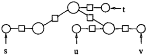
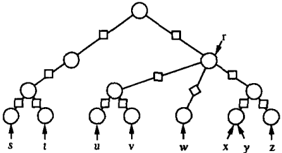
As an example for motivating the introduction of yet another propagation method, consider the junction tree in Figure 1, with evidence e = { s, t, u, v , w, x, y, z } entered as indicated.

Suppose you want to perform a conflict analysis (Jensen, Chamberlain, Nordahl & Jensen 1991). Then you first calculate

If conf is well above 0, it is an indicaiton that the ev­ idence is conflicting. The next thing you would like to do is to trace the conflict further down. You may for example want to "retract" some of the evidence and calculate the conflict measure for the remaining evidence. You may also want to investigate whether

it is the group of findings {x,y,z} which is in con­ flict with the rest. To do so you need probabilities of the type P(e'), where e' is a subset of e. There is a straightforward way to calculate these probabilities, namely to enter e' as evidence, and then most prop­ agation algorithms will provide P(e') as a side effect. However, this is clumsy and time-consuming. There­ fore you may be willing to pay an overhead in time and space for a propagation method which gives you a more direct access to probabilities of subsets.

In this paper we shall present a propagation method which we call cautious propagation. It provides very easy access to P(e') for more subsets than any other propagation method known to the author, and ex­ tended with cautious evidence entering it provides a very fast way of calculating the impact on a hypothe­ sis if a finding as retracted or changed from one value to another.

Cautious propagation is a modification of HUGIN propagation (Jensen, Lauritzen & Olesen 1990) to a message passing design like Shafer-Shenoy propagation (Shafer & Shenoy 1990). We call it cautious propa­ gation because it works in a way not destroying the original tables in the junction tree. Cautious evidence entering was proposed by Dawid (1992) as fast retrac-

tion, however, in his setting it only provided fast re­ traction in special cases.

We start with a closer analysis of the HUG IN propaga­ tion algorithm to pin-point its drawback with respect to calculation of P (e')s, and cautious propagation is defined together with its proof of correctness. Then cautious evidence entering is defined, and we compare the time and space complexity of HUGIN and cau­ tious propagation. Finally, it is illustrated how cau­ tious propagation can be used for sensitivity analysis.

2 P(e')s provided by HUGIN propagation

HUGIN propagation is performed in two phases, a CollectEvidence phase, where messages are sent from the leaves to a chosen root, and a DistributeEvidence phase, where messages are reversed. The content of the messages is explained below.

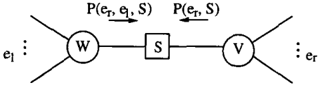
Consider the situation in Figure 2. Assume that the junction tree is consistent before the evidence is en­ tered (for each clique V its table is P (V), and for each separator S its table is P (S)), and let the evidence e be divided by S into e1 and er.

If CollectEvidence is called in a node at the left of W, the table to be transmitted from V to S is P (en S), and PJ:tsfl is transmitted further to W to be multi­ plied to P (W). When later DistributeEvidence is acti­ vated, the table transmitted from W to S is P (er, e1, S) and P�(·��e,'sfl is transmitted to V and multiplied to V 's table (§ is set to 0).

This gives us a way to calculate probabilities for sub­ sets of the evidence at each separator. Since S initially holds P (S), we have at our disposal at S the three ta­ bles P (S),P (enS) and P (er,e�,S). Then

Since er is independent of e1 given S we have

This yields a formula for the calculation of P (e1):

Unfortunately it can only be used if P (er, s) =f. 0 for all states s of S. If P (er, s) = 0 the fraction is put at 0, and the sum is only a lower bound for P (e1) (If we for these states put the fraction to P (s) we also get an upper bound for P (el)). The problem is that the clique tables P (V) are affected by the propagation, and if O 's are introduced you cannot restore the table.

3 Cautious propagation

Consider Figure 2 again and observe that in the DistributeEvidence phase, P (V, er) is multiplied by P�(·�:�.'sfl. If instead we multiply by P (e1 I S) the only difference will be multiplications for configurations s, where P(s, er) = 0. In that case the corresponding en­ tries in P (V, er) are also 0. So multiplying by P ( e1 I S) will give exactly the same result as the HUGIN prop­ agation will give.

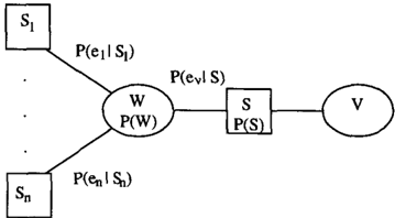
Therefore, the idea behind cautious propagation is that in the CollectEvidence phase let S keep P (S), and store P (W) and P (er I S) separately near W. Now, assume that W has received and stored the mes­ sages P(e1 I S1), . . . , P (en I Sn) (see Figure 3) where ew = el u ... u en.

Then

and

If W is the root, Figure 3 describes the situation af­ ter CollectEvidence(W), and recursively it will in the DistributeEvidence phase be the situation for all non­ leaf nodes.

A more precise description of cautious propagation is the following:

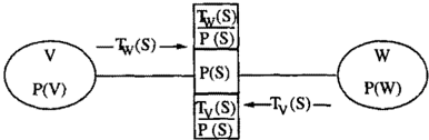
Before evidence is entered, each separator S holds P(S) and each clique V holds P(V) . Whenever S re­ ceives a table Tv(S) from a neighbour W, it is divided by P(S), stored, and a message is sent to the other neighbour clique V (see Figure 4).

Figure 4: A link in a junction tree and the tables stored when a message has been passed in both directions.

A clique W can send a table to a neighbour separa­ tor S if it has received a message from all its other neighbouring separators 81, ... , Sn. The table sent is

For the correctness of the method we see from the considerations above that it is enough to show that Tv(S) = P(S, ew ) , where ew is the evidence entered at the subtree containing Sand W, but not V:

If W is a leaf then

If Tw(Si) = P(Si, ei) then Tl;k�)) = P(ei I Si), and because e1, ... , en are independent given W we have (see Figure 3)

Therefore

4 Cautious entering of evidence

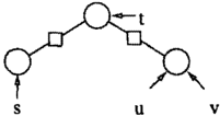
Consider the situation in Figure 5. We can access the complement of s. However, with the present tech­ niques we cannot access the complements of {t}, {u}, and { v}. Fortunately there is an easy way out: Add dummy variables such that findings are always inserted to a leaf in the junction tree, and such that at most one finding is inserted in any node. The construction is illustrated in Figure 6.

Figure 6: Now the probability of all complements of single findings can be accessed by cautious propaga­ tion.

This structural way of accessing complements of single findings through propagation can be achieved simpler by the following modification of the way that findings are inserted: Instead of changing the table in the clique when inserting the finding f, consider the finding as a message Ft, store it, and treat it in the same way as ta­ bles from neighbour separators. This way of handling findings corresponds to the one suggested by Dawid (1992).

Dawid used it in connection to the HUGIN propaga­ tion method to get P(x I e \ {x}). However, O's can mess it up and in order for this to work always you have to use cautious propagation.

In the following we include cautious entering of evi­ dence in the term cautious propagation.

5 P ( e' ) s provided by cautious propagation

LetS be any separator. S divides the evidence e into two sets er and e1, and cautious propagation provides both P(er) and P(e1). Hence we for the situation in Figure 1 have access to the probability of the following

sets:

Let V be a clique with findings It, . . . , f m entered and with adjacent separators 81, ... , Bn. Let ei denote the evidence entered to the subtree containing Si but not V. Take for example the set e1 U e2 U {fi } . Then

and all the factors in the product are available local to V. Therefore P( e1 U e2 U {It}) is easy to calculate.

In general, cautious propagation gives access to the probability of any union of the sets {!I}, . . . , { f m} , el, 0 0 0 'en.

In Figure 1 we therefore also get access to the proba­ bility of

6 Complexity of cautious propagation

We shall compare cautious propagation (with cautious entering of evidence) and HUGIN propagation, which is the fastest known updating method (Shachter, An­ dersen & Szolovits 1991).

Let the junction tree have n cliques (and n - 1 separa­ tors), and assume that all cliques in the junction tree shall receive evidence.

The space requirements for cautious propagation is two extra tables for each separator and a way to store ev­ idence. This will never require more than two times the space as for HUGIN propagation (most often con­ siderably less).

As described in Section 3 cautious propagation re­ quires the junction tree to be consistent before evi­ dence is entered. This can be achieved by a HUGIN propagation; however, it may also be done by cautious propagation with tables of 1 's in the separators. In this case, cautious propagation corresponds exactly to the propagation method suggested by Shafer & Shenoy (1990). When the propagation has terminated, the ta­ bles P(S) for separators and P (V) for cliques can be calculated from the tables stored (we shall revert to this later) .

The methods are composed of the table operations marginalization, multiplication and division. To get insight into the time complexity of the methods we ig­ nore that the time for the operations varies with table sizes. However, multiplication of n tables is counted as n -1 multiplications.

There are the following phases in the calculation of new probabilities:

1. Entering of evidence.
2. Propagation.
3. Calculation of marginals.
4. Reinitialization: Prepare the junction tree for a new set e' of evidence. That is, all tables shall be conditioned on the evidence e just entered. This phase is redundant when the case is closed, and also when there is no need for distinguishing be­ tween the two sets e and e' of evidence.
5. Re b) For both methods there are two marginalizations and two divisions for each link. For the multipli­ cations we have

Re a) HUGIN: n multiplications.

Cautious: No operations.

HUGIN (including entering of evidence):

Two multiplications for each clique except the root, where only one multiplication is necessary, 2n -1.

Cautious:

Let V be a clique with k neighbours. When a message has to be sent along a link, the table for V shall be multiplied with k -1 tables. In order to take care of all messages sent from V we need k(k - 1) multiplications. For the entire propaga­ tion we therefore need

propagations.

To analyse what that means, assume that m cliques in the junction tree have k neighbours and the remaining n - m cliques are leaves. Since the graph is a tree we have2(n-1) = km+(n-m) and we get m = k=�. This gives Multc = k(n -2).

So, in the worst case k = n - 1 and Multc = (n- 1)(n2); in the best case we have Multc = 2(n -2).

For the rest of this analysis we assume that k = 6 (few junction trees are more heavily branched).

The operations above are performed on clique ta­ bles where findings have been entered. To es­ tablish this, the findings are multiplied on auxil­ iary tables. This expands the space requirement,

so that it altogether is twice the requirement for HUGIN propagation.

Re c) The number of propagations are the same. We assume the number of variables to be 6n, which gives 6n marginalizations.

Furthermore cautious propagation requires two multiplications for each link.

• Re d) There is really nothing to do here in HUGIN prop­ agation. What should be done is the normaliza­ tion of all tables by dividing by P(e), however, this can be postponed till later when table op­ erations are performed. In cautious propagation the clique tables are calculated under c). For the separator tables we have (see Figure 4)

So the three tables stored are multiplied. This re­ quires 2(n- 1) multiplications. Normalization is treated in the same way as for HUGIN propaga­ tion.

Counting koefficients of n the complexity of HUGIN propagation amounts to 13n, and under the assump­ tions made the complexity of cautious propagation is 2ln. So, altogether cautious propagation will very sel­ dom take more than twice the time of HUGIN propa­ gation.

7 An application: Sensitivity analysis

Sensitivity analysis is part of explanation, which has to do with explaining to a user how the system has ar­ rived at its conclusions. Explanation for Bayesian net­ works has been studied systematically by Suermondt (1992), and Madigan & Mosurski (1993) have imple­ mented various explanation facilities. Some of the questions to answer in connection to explanation con­ cern the sensitivity of the conclusions to the particular evidence.

Let h be a hypothesis (in the form of a particular con­ figuration of states for some hypothesis variables), and let e be the evidence entered. That is, P(h I e) has been calculated, and now you would like to analyse the relation between the evidence and resulting probabil­ ity.

Definitions: Let e be evidence, h a hypothesis, and let (h, fh, (}3 be predefined thresholds. Evidence e' � e is

• -minimal sufficient if e1 is sufficient , but no proper subset of e 1 is so
• -crucial if e' is a subset of any sufficient set
• -decisive if P(h I e') > 1 03

As can be seen from the definitions above, the heart of sensitivity analysis is to calculate P(h ! e') for subsets e1 of e. If e is not a very small set we cannot hope for an easy way of calculating P(h I e 1 ) for all subsets. However, with cautious propagation (and cautious en­ tering of evidence) the probability for a crucial number of subsets can be achieved.

Cautious propagation yields P(e') for subsets as de­ scribed in Sections 3 and 4. Now, enter has evidence to a clean junction tree, and HUGIN propagate such that all tables are conditioned on h (this also yields P(h)). Next e is entered cautiously and cautious prop­ agation is performed. This gives access to P(e' I h) for the same subsets as before, and Bayes' formula gives P(h I e'). (Jensen, Aldenryd & Jensen 1995) gives some examples of how cautious propagation can be used in sensitivity analysis.

Another natural set of questions in sensitivity analysis are What-if-questions: If the finding on the variable X had been y instead of x, what would P(h I eU{y}\{x}) be?

This type of question can also easily be answered through cautious propagation and cautious evidence entering. Let namely X be a member of V, and let a finding on X be x. After cautious propagation the situation is, that local to V you have P(V), P(ei I Si) for all adjacent separators Si, and tables Ft for the findings f to multiply on P(V). It is then easy to sub­ stitute Fx with Fy and calculate P(V, e U {y} \ { x}) as the product of all tables local to V, and finally marginalize V out to get P(e U {y} \ {x}). The same is done with the junction tree conditioned on h to get P(e U {y} \ {x} I h), and Bayes' formula yields P(h I e U {y} \ {x}).

Note that the analysis above did not require any extra propagations.

Acknowledgements

Thanks to the ODIN group at Aalborg University (http:www.iesd.auc.dkfodin), in particular to S0ren Dittmer for valuable discussions. Thanks also to S0ren Aldenryd and Klaus B. Jensen for their contributions to the part on sensitivity analysis.

References

• Dawid, A. ( 1992 ) . Applications of a general propa­ gation algorithm for probabilistic expert system, Statistics and Computing 2: 25-36.
• Jensen, F. V., Aldenryd, S. & Jensen, K. B. ( 1995 ) . Sensitivity analysis in bayesian networks, Pro­ ceedings of ECSQARU'95, Fribourg, Switzerland. To appear.
• Jensen, F. V., Chamberlain, B., Nordahl, T. & Jensen, F. ( 1991 ) . Analysis in HUGIN of data conflict, in N.-H. Bonnisone et al. ( ed. ) , Uncertainty in Artificial Intelligence 6, pp. 519-528.
• Jensen, F. V., Lauritzen, S. L. & Olesen, K. G. ( 1990 ) . Bayesian updating in causal probabilistic networks by local computations, Computational Statistics Quarterly 4: 269-282.
• Madigan, D. & Mosurski, K. ( 1993 ) . Explanation in belief networks, Technical report, University of Washington, US and Trinity College, Dublin, Ire­ land.
• Shachter, R. D., Andersen, S. K. & Szolovits, P. ( 1991 ) . The equivalence of exact methods for probabilistic inference on belief networks, Techni­ cal report, Department of Engineering-Economic Systems, Stanford University.
• Shafer, G. & Shenoy, P. ( 1990 ) . Probability propaga­ tion, Annals of Mathematics and Artificial Intel­ ligence 2: 327-352.
• Suermondt, H. J. ( 1992 ) . Explanation in Bayesian Belief Networks, PhD thesis, Knowledge Systems Laboratory, Medical Computer Science, Stanford University, California, Stanford, California 94305. Report No. STAN-CS-92-1417.