Centric Selection: a Way to Tune the Exploration/Exploitation Trade-off

David Simoncini, S´ ebastien Verel Philippe Collard, Manuel Clergue

Abstract

In this paper, we study the exploration / exploitation trade-off in cellular genetic algorithms. We define a new selection scheme, the centric selection, which is tunable and allows controlling the selective pressure with a single parameter. The equilibrium model is used to study the influence of the centric selection on the selective pressure and a new model which takes into account problem dependent statistics and selective pressure in order to deal with the exploration / exploitation trade-off is proposed: the punctuated equilibria model. Performances on the quadratic assignment problem and NK-Landscapes put in evidence an optimal exploration / exploitation trade-off on both of the classes of problems. The punctuated equilibria model is used to explain these results.

1 Introduction

The exploration/exploitation trade-off is an important issue in evolutionary computation. By tuning the selective pressure on the population, one can find an optimal (or near-optimal) tradeoff between exploitation and exploration. In cellular Evolutionary Algorithms (cEAs), the population is embedded on a bidimensional toroidal grid and each solution interacts with its neighbors thanks to a certain neighborhood. The convergence rate of the algorithm is then dependent of the shape and size of the grid and of the neighborhood. The smallest symetric neighborhood that can be defined is the well-known Von Neumann neighborhood of radius 1. It guarantees a slow isotropic diffusion of genetic information through the grid. But when solving complex multimodal problems, it is necessary to slow down even more the propagation speed of the best solution because the algorithm still often converges over a local optimum.

Our goal in this paper is to establish a relation between the selective pressure on the population and the effects of recombination and mutation operators, in order to find an optimal exploration/exploitation trade-off. To do so, we propose a new selection scheme able to control the selective pressure and a theoretical model which takes into account the effects of stochastic variations on an optimization problem. In section 2 we define a selection scheme able to

tune the selective pressure and present the algorithm used in the experiments. In section 3, we analyze the selective pressure with respect to the selection method and present a new model which takes into account the stochastic variations. In section 4 we present performances on Quadratic assignment problem instances and on NK-Landscapes and we explain the results with the model proposed.

1.1 Cellular Evolutionary Algorithms

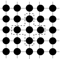
A cellular Evolutionary Algorithm (cEA) [23] is an EA in which the population is embedded on a bidimensionnal toroidal grid (see figure 1). Each cell of the grid contains a solution. Embedding the solutions on a grid allows defining a neighborhood between the cells. The most commonly used one in cEAs is the Von Neumann neighborhood (shown on figure 1). At each generation, every cell on the grid is updated by selecting parents in its neighborhood and applying stochastic operators such as crossover and mutation. Several strategies exist, synchronous and asynchronous, to update the cells. The small overlapped neighborhoods guarantee the diffusion of solutions through the grid [18]. Such algorithms are especially well suited for complex problems [9] and are of advantage when dealing with dynamic problems [20].

1.2 Selective pressure

One of the main properties that differs between EAs and cEAs is the rate of convergence (propagation speed of the best solution) : It is exponential for EAs and quadratic for cEAs. Therefore, the selective pressure on the population is weaker for a cEA than for an EA. Controlling the selective pressure is critical since it can avoid premature convergence of the algorithm when solving complex multimodal problems. Several parameters related to the selective pressure can prevent the algorithm from getting stuck in a local optimum. The topology of the grid, the local neighborhood, the properties of the selection operator are such parameters. By correctly tuning these parameters for a given problem, one can find a good exploration/exploitation tradeoff and minimize the risks of premature convergence. Sarma et al. established a link between the radius of the

neighborhood and the radius of the grid : changing this ratio directly affects the selective pressure on the population [16]. Alba et al. analyzed performances of cEAs with a fixed size neighborhood and different grid shapes. They arrived to the conclusion that thin grids are well-suited for complex multi modal problems and large grids are well-suited for simple problems. The main explanation is that thinner grids give lower selective pressure [3]. Takeover times and growth curves analysis are useful to measure the selective pressure on a population, but it is not sufficient to decide of a trade-off between exploration and exploitation: it is necessary to include effects of the stochastic variations due to the operators in the analysis. Janson et al. proposed a hierarchical cEA which allows achieving different levels of exploration /exploitation tradeoff in distinct zones of the population simultaneously [8].

A standard technique to study the induced selective pressure without introducing the perturbing effect of variation operators is to let selection be the only active operator, and then monitor the number of best solution copies in the population [6]. The takeover time is the time needed for one single best solution to colonize the population with selection as the only active operator. Let λ be the size of the population, t the number of generations and N ( t ) the number of best solution copies at generation t . The population is initialized with one solution of good fitness and λ -1 solutions of null fitness. Since no other evolution mechanism but selection takes place, the good fitness solution spreads over the grid. The takeover time is then the smaller time t such that N ( t ) = λ . Analysing the growth of N ( t ) as a function of t also gives an indication on the selective pressure. It shows the convergence rate of the algorithm when selection is the only active operator. When the slope of the growth curve of N ( t ) is low, the convergence rate is low and the takeover time is high. On the other hand, a high slope of the growth curve leads to a short takeover time. In the first case, the selective pressure on the population is weaker than in the second case.

1.3 Growth curves and takeover time models

Characterizing the growth curves and the takeover time is an important issue in the study of the selective pressure [6]. Many models have been proposed to define the behaviour of structured population evolutionary algorithms. Sarma and De Jong proposed a logistic model in which the coefficient of the growth curve of the best solution is shown to be an inverse exponential of the ratio between radii of the neighborhood and the underlying grid [16]. This conclusion was guided by an empirical analysis of the effects on the convergence rate and the takeover time of several neighborhood sizes and shapes. Sprave proposed a hypergraph based model of population structures and a method for the estimation of growth curves and takeover times based on the probabilistic diameter of the population [19]. Gorges-Schleuter proposed a study about takeover time and growth curves for cellular evolution strategies. She obtained a linear model for ring populations and a quadratic model for a torus population structure [7]. Several authors wrote about theoretical or empirical models of growth curves

and takeover time. Giacobini et. al. proposed a model for cellular evolutionary algorithms with asynchronous update policies [4]. He summarized his results and proposed models for synchronous updates [5] that will be evoked later in this paper. Alba proposed a model for distributed evolutionary algorithms consisting in the sum of logistic definition of the component takeover regimes [2]. In his paper, he made an interesting review of existing models and compared two of them (the logistic model and the hypergraph model) with his newly proposed one. For a detailed state of the art of cEAs, see [1].

2 Centric selection

In this section we present a new selection scheme for cEAs that allows tuning accurately the selective pressure.

Algorithm 1 Centric Selection algorithm

CentricSelection index: int, β : double neighbors ←-GetNeighborhood(index) candidate 1 ←-Select(neighbors, β ) candidate 2 ←-Select(neighbors, β ) Best( candidate 1 , candidate 2 )

The centric selection (CS) idea is to change the probability of selecting the center cell of the neighborhood. This scheme allows slowing down the convergence speed while keeping an isotropic diffusion of good solutions through the grid. The CS is a determinist tournament selection. But unlike the standard deterministic tournament, cells in the neighborhood may have different probabilities of being selected for the competition. The anisotropic selection [17] is another selection scheme which modifies the probability of selection a cell for a deterministic tournament. With the anisotropic selection, the diffusion of solutions is not isotropic, so we propose the CS which is easier to study. We have p c = β the probability of selecting the center cell and p n = p s = p e = p w = 1 4 (1 -β ) the probability of selecting either north, south, east or west cell. When β = 1 5 , all cells have the same probability of being selected for the competition: this particular case of CS is the standard binary tournament selection. When β = 1, only the center cell can be selected for the tournament: in this particular case where the same solution is selected two times, the crossover operator is not applied in the cEA. Only mutations are applied to the solution, and with an elitist replacement strategy, the algorithm behaves as the parallelisation of as many hill climbers as there are solutions in the population. The CS is described in algorithm 1. The candidates compete in a deterministic tournament returning the best one. For each cell on the grid, two parents are selected per generation, as we can see in the algorithm 2. Stochastic variations operators are applied to the parents, generating two children. The replacement strategy is elitist: the best child replaces the current solution on the grid if it has a better fitness. The use of a temporary grid is necessary for a synchronous update of the cells.

Algorithm 2 Description of our cEA

cEA population: vector, β : double tempGrid: vector while continue() do for i = 1 to GridSize do parent 1 ←-CentricSelection(i, β ) parent 2 ←-CentricSelection(i, β ) ( child 1 , child 2 ) ←-Crossover( parent 1 , parent 2 ); Mutate( child 1 ) Mutate( child 2 ) tempGrid[i] ←-Best( population [ i ], child 1 , child 2 end for Replace(population, tempGrid)

) end while

3 Modeling cEAs

In this section, we present two models of the search dynamic in cEAs. In the first one, the Equilibrium Model (EM) we consider that the optimal solution has been found and observe how it colonizes the grid. This model is classical in the studies on the selective pressure and one the exploration/exploitation tradeoff. The informations given by this model are takeover times and best solution growth curves. As the stochastic variations operators are not taken into account, the same dynamic occurs in experimental runs when the recombination and mutation operators are ineffective: when the system has reached an equilibrium.

In the second one, we consider that a better solution can be found with a certain probability and observe the frequency of apparition of this new solution with respect to our algorithm's parameters. It is a model of the transition between two periods of fitness stability. We call this new model the Punctuated Equilibria Model (PEM).

3.1 Equilibrium model

In order to measure the selective pressure induced by the CS, we observe what happens when no more solution improvement is possible. In this case, crossover and mutation are no longer useful and the evolution process has reached an equilibrium. Hence, we observe the time needed for a single best solution to conquer the whole grid, and look at the growth curve obtained and the takeover time.

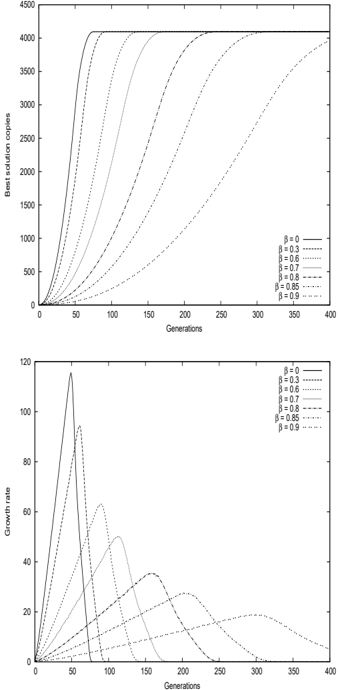
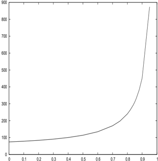
We measure the effects of CS on selective pressure by observing these growth curves and takeover times on a square grid of side 64. Figure 2 shows the takeover time as a function of β . The takeover time is not defined for β = 1. The selective pressure drops when the value of β increases. We can see on figure 3 the growth of the number of copies of the best solution in the population (top) and its growth rate (bottom). There are two stages in the shape of the

curve. The growth rate is linear in the first part and quadratic in the second part. When using this selection scheme, the diffusion of the best solution is still isotropic. So the best solution roughly propagates describing an obtuse square as long as no side of the grid is reached. This corresponds to the first part of the growth rate curve. Once the sides are reached by some copies of the best solution, the dynamic changes as we can observe on the second part of the growth rate curves.

3.2 Punctuated equilibria model

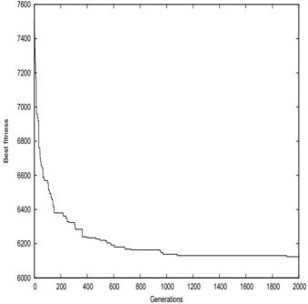
In this section, we propose a new model which will help in the understanding of the search dynamics of an Evolutionary Algorithm. This model was first designed for a cellular EA but can be easily extended to any kind of evolutionary algorithm. We consider a cEA initialized with random solutions. We make sure that the best solution in the population is unique. Our goal is to simulate an evolutionary run: We simulate recombination and mutation operators with probabilities that the mating is efficient or not (i.e. produces a new best solution). We consider three different types of matings: between two copies of the best solution (mating 11), between one copy of the best solution and one suboptimal solution (mating 01) and between two sub-optimal solutions (mating 00). We introduce probabilities P 11 , P 01 and P 00 that matings of type 11, 01 and 00 produce a new best solution, fitter than the previous best one. Figure 4 is an example of evolutionary run on some optimization problem (minimisation task). We can see that there are some stagnation periods where the best solution don't improve. Then, an amelioration occurs and the population enters another stability period. An evolutionary run is a sum of stagnation periods and punctual improvements. Our punctuated equilibria model computes the

probability of improving the best solution in the population according to the variables described above.

With this model, the probability of finding a new best solution at a given generation t is :

where n 00 ( t ), n 01 ( t ) and n 11 ( t ) are the number of matings of each type for the generation t .

which gives:

1 In the following equations, we only denote the dependance on β for P and Σ ij for readability.

The average time to find a new best solution is given by :

The performance of an algorithm can be measured by the time E needed to find a new best solution but also by the probability P of improvement in a preset time T . We have the probability of improving the best solution in T generations :

with Σ ij ( T ) = ∑ T t =1 n ij ( t ) the sum over T of mating of each type.

The parameters P ij are problem dependent and the values of Σ ij are given by the selection scheme used. The selection process is usually controlled by a parameter such as the tournament size or in the case of the CS: β . This parameter should be used to maximize the probability 1 P . Intuitively, the ideal selection process maximizes the Σ ij which have the higher P ij . More precisely, assuming that the control parameter of the selection process is β , the parameter β ∗ which maximizes the probability P ( T ) verifies:

If it is possible to have a model of Σ ij ( β ), it would be possible to calculate the optimal β as a function of P ij .

In this model, the exploration/exploitation tradeoff is given by the number of each possible matting (00, 01 and 11). The model could be used to explain the probability and the time to find a new best solution according to the selective pressure, and also to tune the value of parameters which have an impact on the selective pressure, such as β , to have the highest probability to evolve toward a new best solution. Equation 1 gives precisely the best exploration and exploitation tradeoff and allows computing the optimal value of β (in our case) for this trade-off. In the following, we will show the validity of the PEM on some optimization problems.

4 QAP and NK landscapes

In this section, we study the effect of selective pressure on performances through experiments of a cEA with CS on two well-known classes of problems. The optimal exploration / exploitation tradeoff found will be explained thanks to the PEM presented in the previous section.

4.1 Problems presentation

The problems proposed, Quadratic Assignment Problem and NK landscapes, are known to be difficult to optimize. The important number of instances of the Quadratic Assignment Problem and the tunable parameters of the NK landscapes allow managing the difficulty of the problems.

4.1.1 Quadratic Assignment Problem

This section presents the Quadratic Assignment Problem (QAP) which is known to be difficult to optimize. The QAP is an important problem in theory and practice as well. It was introduced by Koopmans and Beckmann in 1957 and is a model for many practical problems [11]. The QAP can be described as the problem of assigning a set of facilities to a set of locations with given distances between the locations and given flows between the facilities. The goal is to place the facilities on locations in such a way that the sum of the products between flows and distances is minimal. Given n facilities and n locations, two n × n matrices D = [ d kl ] and F = [ f ij ] where d kl is the distance between locations k and l and f ij the flow between facilities i and j , the objective function is :

where p ( i ) gives the location of facility i in the current permutation p . Nugent, Vollman and Ruml proposed a set of problem instances of different sizes noted for their difficulty [14]. The instances they proposed are known to have multiple local optima, so they are difficult for an evolutionary algorithm. The best algorithm known is the fast hybrid evolutionary algorithm [13] which combines an evolutionary algorithm with an improvement of the fast tabu search of Taillard.

Set up

We use a population of 400 solutions placed on a square grid (20 × 20). Each solution is reprensented by a permutation of N where N is the size of a solution. The algorithm uses a crossover that preserves the permutations:

• Select two solutions p 1 and p 2 as genitors.
• Choose a random position i .
• Find j and k so that p 1 ( i ) = p 2 ( j ) and p 2 ( i ) = p 1 ( k ).
• exchange positions i and j from p 1 and positions i and k from p 2 .
• repeat N/ 3 times this procedure where N is the size of an solution.

This crossover is an extended version of the UPMX crossover proposed in [12]. The mutation operator consists in randomly selecting two positions from the solution and exchanging those positions. The crossover rate is 1 and we do a mutation per solution. We perform 200 runs for each tuning of the two selection operators. An elitism replacement procedure guarantees the solutions stay on the grid if they are fitter than their offspring.

4.1.2 NK landscapes

The NK landscapes were proposed by Kaufmann to model the boolean network and used in optimisation in order to explore how epistasis is linked to the ruggedness of search spaces [10]. Epistasis corresponds to the degree of interactions between the 'loci' of a solution and ruggedness is the number of local optima of the search space. The main characteristic of NK Landscapes is that they allow tuning the epistasis level with a single parameter K . The parameter N determines the length of the solutions.

The fitness of solutions for a NK landscape is given by the function

defined on binary strings of length N . Each binary string is a solution with N locations. An atom with fixed epistasis level is represented by a fitness component

associated to each bit i . It depends on the value of the bit i and on the value of K other bits of the string ( K must fall between 0 and N -1). The fitness f ( x ) of x ∈ { 0 , 1 } N is the average of the values of the N fitness components f i :

where { i 1 , ..., i k } ⊂ { 1 , ..., i -1 , i + 1 , ..., N } . Many ways have been proposed to choose the K other locations from the N of the solutions. The mainly used ones are adjacent and random neighborhoods. With the first one, the K nearest locations of the location i are chosen (the solution is taken to have periodic boundaries). With the random neighborhood, K locations are randomly selected from the solution. Each fitness component f i is specified by extension, ie a random number y i, ( x i ,x i 1 ,...,x ik ) from [0 , 1] is associated with each element ( x i , x i 1 , ..., x ik ) from { 0 , 1 } K +1 . Those numbers are uniformly distributed in the interval [0 , 1].

Set up

The size of the population is 400 solutions. The crossover used is a one point crossover, applied with a probability of 1. The mutation is a bit flip applied with a probability of 1 n where n is the size of a solution. We perform 200 runs for every parameter set, and each run stops after 1500 generations. Runs are performed on instances of sizes N = 32, with K ∈ 2 .. 12.

4.2 Performances

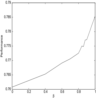
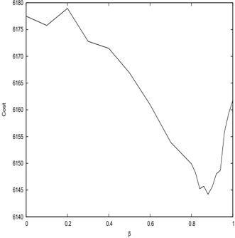
Figure 5 and table 1 show performances of a cEA using CS on some QAP instances of various sizes. The instance in figure 5 is a well-known instance of size 30. The first fact that we notice when looking at these results is that there is an optimal setting, different from the extreme values 0 and 1 for the parameter β . This indicates that for a certain setting of the parameters, and thus for a certain selective pressure, the search dynamic leads to optimal results. Curves representing the instances summarized in table 1 have the same shape as figure 5. On each instance, the optimal value of β is around 0 . 85. The performances increase up to these values and then decrease. Performances of CS are significantly better than the one obtained with a cEA using standard binary tournament selection. The standard cEA is observable on the curve at the points β = 0 . 2 and is reported in the table 1. We can also notice in table 1 that the standard deviation is lower for the optimal value of β than with a cEA with binary tournament selection.

Table 1: Avg. results and std.dev.on QAP instances

Instance	Std cGA	Best avg. results	Opt. β
Nug30	6178 [28]	6144 [14]	0 . 88
Tai40a	3 . 23 × 10 6 [14343]	3 . 21 × 10 6 [12000]	0 . 84
Sko42	15969 [75]	15909 [34]	0 . 82
Tai50a	5 . 092 × 10 6 [20721]	5 . 080 × 10 6 [13372]	0 . 82
Tai60a	7429118 [27760]	7385390 [19391]	0 . 86

Figure 6 and table 2 present performances of a cEA with CS on some instances of NK landscapes. Parameters of the landscapes are N = 32 and K = 10 for the figure 6 and are summarized in table 2 for the other instances.

We can see that the shape of the performances' curve is different from the QAP curve. The performance increases until β reaches its maximum value. The same results are obtained for all the instances in table 2. The parameter K tunes the difficulty of the instance. We can see that for K = 2, there is no optimal value for β . The reason is that the optimum is always found. For K = 4, the standard cEA sometimes get stuck in a local optimum, and with β = 1 our algorithm always find the optimum. On every instance, except K = 2, the optimal value for β is 1.

However, this value β = 1 is a particular one, since it breaks all communications on the grid. As long as the value of the parameter increases, the chances of selecting two different solutions for recombination decrease. For β = 1, the algorithm is the parallelisation of as much hill climbers as there are cells on the grid : It constantly selects the center cells of the neighborhoods, so there is no crossover and any amelioration is due to a bit flip.

Table 2: Avg. performances and std.dev.on NK instances with N = 32

K	Std cGA	Best avg. results	Best β
2	0 . 734329 [0]	0 . 734329 [0]	[0 , 1]
4	0 . 79597 [0 . 003]	0 . 798197 [0]	1
6	0 . 782934 [0 . 01]	0 . 799124 [0 . 003]	1
8	0 . 771277 [0 . 01]	0 . 789103 [0 . 004]	1
10	0 . 763510 [0 . 01]	0 . 785115 [0 . 003]	1
12	0 . 750043 [0 . 01]	0 . 774479 [0 . 009]	1

So the best setting for CS can be compared to the parallelisation of as many hill climbers as there are cells on the grid. The parallelisation of hill climbing seems to be a good algorithm for solving NK landscapes problems, which could be explained by the size of basins of attraction [21] and [15].

4.3 Probabilities of discovering better solutions

In order to explain the optimal values of β for QAP and NK-Landscape and to validate the PEM, we compute P , the probability of discovering a new best solution in the population taken from the PEM, with real data. We calculated it for one instance of QAP and one instance of NK-Landscapes. With this calculation we want to find the value of β that maximizes the probability of discovering a new solution. This probability depends on the value of Σ ij , and thus on time: if at a generation t no new solution is discovered, the actual best solution spreads in the population according to the selective pressure. If during an interval of time corresponding to the takeover time no new solution

is discovered then the population converges. We can compute the ideal β value for a given number of generations T because Σ ij ( T ) relies on β and on time: after T generations Σ ij ( T ) is different according to β , and for the optimal value of β Σ ij ( T ) leads to the best probability P .

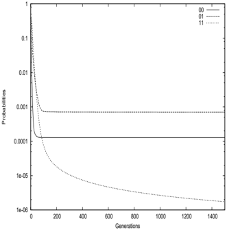
We estimated the Σ ij with the same experiments done to compute growth curves and takeover time. We averaged the number of matings of each type at each generation over 10 3 runs. Then, we needed to know the probabilities P 00 , P 01 and P 11 . We estimated these probabilities using a Bayesian process during the runs. We averaged the values obtained by generations over 500 runs. Figure 7 shows the result of the estimation of probabilities on the QAP instance Nug30. The ordonate scale is logarithmic because of the variations of probabilities. The curves representing the P ij intersect, so the value of β which maximizes P may change during a run. We computed P with estimated values of P ij taken by steps of 50 generations. The values of Σ ij are also generation dependent. For each value of β , we took the Σ ij value after 100 generations: that is Σ ij (100). During a run, it would correspond to allowing a stagnation period of 100 generations before stopping the run, which is reasonnable.

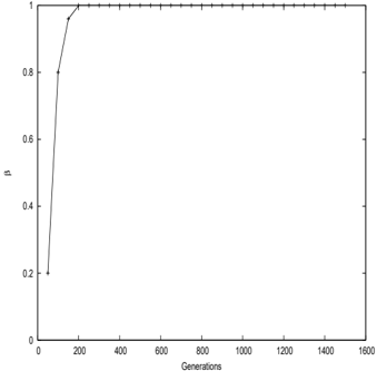
The figure 8 shows the optimal values of β as a function of generations for the QAP instance Nug30. During the first 700 generations, the optimal value is β = 0 . 2. Then, there is a transition of approximatively 150 generations. During this phase, the ideal value of β grows until it reaches 1. In our experiments, we observe optimal values of β between 0 . 8 and 0 . 9 according to the QAP instance. Values of β are constant during the runs. But the PEM shows that the selective pressure should be strong at the beginning (low values of β ) and then weak (high values of β ). If β is constant, intermediate values in the range [0 . 8 , 0 . 9] give the best average selective pressure for QAP instances.

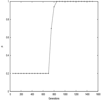
The figure 10 shows the optimal values of β as a function of generations for

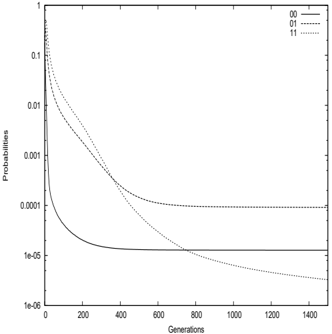
a NK-Landscape with N = 32 and K = 10. We can see that the optimal β value increases fastly and reaches 1 in the early generations. The ideal selective pressure is weak, and it is not surprising that the best performances are obtained when β = 1 in our experiments. Figure 9 shows the estimation of P ij as a function of generations. We can see that the curve representing P 11 drops down very fast. With a negligible probability of improving the current best solution with mutations, there is no sense in spreading this solution. With β = 1, the current best solution in the population cannot spread.

The PEM has been used in order to explain the exploration / exploitation

trade-off on two different classes of problems. Coupled with the centric selection, it showed the ideal selective pressure along the search process. This model can be used to tune any parameter which has some influence on the number of matings of each type defined in the previous section. The computation cost is low, since the estimation of probabilities by a Bayesian process is precise: we averaged the estimation on 500 runs but the standard deviation was low ( ≈ 10 -6 ).The Σ ij are only computed once since they are independent from the optimization problem tackled.

5 Conclusion

The exploration/exploitation trade-off is an important issue in evolutionary algorithms. In this paper, we propose a model that takes into account stochastic variations and improvement of the quality of the solutions, the punctuated equilibria model. In order to study the exploration / exploitation trade-off we propose a tunable selection operator: the centric selection. By monitoring the probability of selecting the center cell of neighborhoods for a tournament selection, this selection operator allows tuning accurately and continuously the selective pressure with one single parameter ( β ). The performance results on QAP instances and NK-Landscapes showed different optimal settings of the centric selection, and thus different ideal selective pressures. Using the punctuated equilibria model, we put in evidence the optimal values of the centric selection's control parameter observed on QAP instances and NK-Landscapes. The punctuated equilibria model also put in evidence that the ideal selective pressure is not constant during the search process in the case of QAP instances.

In this paper, we used the PEM in order to explain experimental results. In future works, we will use it in order to predict optimal exploration / exploitation trade-offs and to adapt the selective pressure during the runs. To do so, we will both estimate the P ij and tune the selection operator online during the search process. The centric selection will be used in auto-adaptative algorithms with the advantage of modifying the exploration / exploitation ratio with a single parameter. It will also be applied on real problems and compared to other optimization methods.

References

1. E. Alba and B. Dorronsoro. Cellular Genetic Algorithms . Springer-Verlag, 2008.
2. E. Alba and G. Luque. Growth Curves and Takeover Time in Distributed Evolutionary Algorithms. In K. D. et al., editor, Genetic and Evolutionary Computation Conference (GECCO-2004) , volume 3102 of Lecture Notes in Computer Science , pages 864-876, Seattle, Washington, 2004.
3. E. Alba and J. M. Troya. Cellular evolutionary algorithms: Evaluating the influence of ratio. In PPSN , pages 29-38, 2000.
4. M. Giacobini, E. Alba, and M. Tomassini. Selection intensity in asynchronous cellular evolutionary algorithms. In GECCO , pages 955-966, 2003.
5. M. Giacobini, M. Tomassini, A. Tettamanzi, and E. Alba. Selection intensity in cellular evolutionary algorithms for regular lattices. IEEE Trans. Evolutionary Computation , 9(5):489-505, 2005.
6. D. E. Goldberg and K. Deb. A comparative analysis of selection schemes used in genetic algorithms. In FOGA , pages 69-93, 1990.

1. M. Gorges-Schleuter. An analysis of local selection in evolution strategies. In GECCO , pages 847-854, 1999.
2. S. Janson, E. Alba, B. Dorronsoro, and M. Middendorf. Hierarchical cellular genetic algorithm. In J. Gottlieb and G. R. Raidl, editors, Evolutionary Computation in Combinatorial Optimization EvoCOP , volume 3906, page 111.122, 2006.

1. K. A. D. Jong and J. Sarma. On decentralizing selection algorithms. In ICGA , pages 17-23, 1995.
2. S. A. Kauffman. The Origins of Order . Oxford University Press, New York, 1993.
3. T. Koopmans and M. Beckmann. Assignment problems and the location of economic activities. Econometrica , 25(1):53-76, 1957.
4. V. Migkikh, E. Topchy, V. Kureichik, and E. Tetelbaum. Combined genetic and local search algorithm for the quadratic assignment. In Proceedings of the SecondAsia-Pacific Conference on Genetic Algorithms and Applications (APGA , pages 144-151, 2000.
5. A. Misevicius. A fast hybrid genetic algorithm for the quadratic assignment problem. In GECCO '06: Proceedings of the 8th annual conference on Genetic and evolutionary computation , pages 1257-1264, 2006.
6. C. Nugent, T. Vollman, and J. Ruml. An experimental comparison of techniques for the assignment of techniques to locations. Operations Research , 16:150-173, 1968.
7. G. Ochoa, M. Tomassini, S. Verel, and C. Darabos. A study of nk landscapes' basins and local optima networks. In Genetic and Evolutionary Computation - GECCO-2008 , pages 555-562, Atlanta, 12-16 July 2008. ACM.
8. J. Sarma and K. A. De Jong. An analysis of the effects of neighborhood size and shape on local selection algorithms. In PPSN , pages 236-244, 1996.
9. D. Simoncini, S. Verel, P. Collard, and M. Clergue. Anisotropic selection in cellular genetic algorithms. In M. K. et al., editor, Genetic and Evolutionary Computation - GECCO-2006 , pages 559-566, Seatle, 8-12 July 2006. ACM.
10. P. Spiessens and B. Manderick. A massively parallel genetic algorithm: Implementation and first analysis. In ICGA , pages 279-287, 1991.
11. J. Sprave. A unified model of non-panmictic population structures in evolutionary algorithms. Proceedings of the congress on Evolutionary computation , 2:1384-1391, 1999.
12. M. Tomassini. Spatially Structured Evolutionary Algorithms: Artificial Evolution in Space and Time (Natural Computing Series) . Springer-Verlag New York, Inc., Secaucus, NJ, USA, 2005.
13. S. Verel, M. Tomassini, and G. Ochoa. The connectivity of nk landscapes' basins: a network analysis. In Proceedings of Artificial Life XI , pages 648655, 8-5 2008.
14. E. Weinberger. Correlated and un correlated fitness landscapes and how to tell the difference. In Biological Cybernetics , pages 63:325-336, 1990.

1. D. Whitley. Cellular genetic algorithms. In ICGA , page 658, 1993.