Clustering Without (Thinking About) Triangulation

Denise L. Draper ddraper·@cs. washington. edu

Department of Computer Science and Engineering University of Washington, Seattle, WA 98195

Abstract

The undirected technique for evaluating be­ lief networks [Jensen et al., 1990a, Lauritzen and Spiegelhalter, 1988] requires clustering the nodes in the network into a junction tree. In the traditional view, the junction tree is constructed from the cliques of the moral­ ized and triangulated belief network: trian­ gulation is taken to be the primitive concept, the goal towards which any clustering algo­ rithm (e.g. node elimination) is directed. In this paper, we present an alternative concep­ tion of clustering, in which clusters and the junction tree property play the role of prim­ itives: given a graph (not a tree) of clusters which obey (a modified version of) the junc­ tion tree property, we transform this graph until we have obtained a tree. There are sev­ eral advantages to this approach: it is much clearer and easier to understand, which is important for humans who are constructing belief networks; it admits a wider range of heuristics which may enable more efficient or superior clustering algorithms; and it serves as the natural basis for an incremental clus­ tering scheme, which we describe.

1 Introduction

Belief networks are directed acyclic graphs in which nodes represent uncertain variables and arcs be­ tween nodes represent probabilistic interactions be­ tween variables. A belief network is parameterized by providing, for each variable X, a conditional prob­ ability of that variable given its parents in the net­ work, P(XIpa(X)). For variables with no parents in the network a simple prior probability P(X) is pro­ vided. A belief network may be evaluated to give the marginal probability of all variables in the net­ work, possibly conditioned on observations of values of some of the variables. There are several algo­ rithms for evaluating belief networks, but it has been shown [Shachter et al., 1994] that. all known exact al- gorithms are equivalent to the undirected belief net­ work evaluation technique of [Jensen et a/., 1990a, Lauritzen and Spiegelhalter, 1988]. This algorithm works in two stages: in the first. stage a junction tn:e is constructed, and in the second stage, messages are propagated through the junction tree.

We will give a short review of triangulation and junc­ tion tree construction; for more detail see e.g. [Jensen, 1988], [Almond and Kong, 1991], [Kjrerulff, 1990], [Jensen and Jensen, 1994].

Junction trees have traditionally been constructed by the following method:

1. "Moralize" the belief network by adding arcs con­ necting every pair of parents of any variable in the network, and dropping the directions on all arcs.
2. Triangulate the (now undirected) network by adding fill arcs until no chord-less cycles of length greater than three remain.
3. Create a tree whose vertices are the cliques of the triangulated graph and which are connected such that the junction tr·ee proper·ty holds: if any two cliques contain a particular variable V, then every clique on the path between those two cliques must also contain that variable.

Triangulation is usually done by node elimination, which proceeds iteratively as follows:

1. Select a non-eliminated variable X to eliminate.
2. Add fill arcs connecting all the non-eliminated neighbors of X to one another (i.e. make the union of X and its neighbors fully connected).
3. Mark X as eliminated.

When all the variables have been eliminated, the graph is guaranteed to be triangulated.

The cost of a junction tree is the cost of doing the message propagation in that tree, and is proportional to the sum of the sizes of the "potentials" of each clique in the tree. The size of the potentials is the product of the number of states of each variable in the clique. Different choices of fill arcs can gener­ ate junction trees of radically differing cost; minimiz-

ing the cost of a junction tree is NP-complete [Am­ borg et al., 1987]. The most effective known heuristic is the "minimum-weight" heuristic, which eliminates the variable whose non-eliminated neighbors form the clique with the smallest potential [Kjrerulff, 1990].

One difficulty with node elimination, or with triangu­ lation in general, is that it is very difficult to under­ stand. The original graphical structure of the belief network doesn't help much: it is generally very diffi­ cult to determine visually if a graph is triangulated, and seeing the cliques of a triangulated graph is even more difficult, especially when they have large over­ laps. Belief networks are often constructed by people, and given the complexity of belief network evaluation it may be assumed that people are interested in en­ gineering their networks so as to reduce the cost of evaluation. The difficulty of visualizing the clustering process makes such engineering much more difficult.

The work of [Shachter et a/., 1994] and [Jensen and Jensen, 1994] underscores the fundamental importance that triangulation plays in all known belief network evaluation algorithms. But it does not follow that we must think in terms of triangulation-"hidden trian­ gulation" may be just as effective as "overt triangula­ tion."

In the remainder of this paper, we present a new frame­ work for the construction of junction trees, which is not overtly based on triangulation. Section 2 intro­ duces cluster graphs, which are a generalization of junction trees to multiply-connected graphs, and ex­ plains the general principles of transforming a clus­ ter graph into a junction tree. Section 3 enumerates some of the transformations that can be used in this process, and Section 4 combines these transformations into two algorithms: the transformational equivalent of the node elimination algorithm and another com­ pletely new algorithm. Our original motivation in un­ dertaking this research was to find an algorithm for incremental clustering which would allow the dynamic addition of variables and arcs to the belief network without forcing the recomputation of the entire junc­ tion tree, and Section 5 presents an algorithm for in­ cremental clustering which arises quite naturally from our cluster graph framework. Section 6 presents some empirical results on our algorithms, and Section 7 con­ cludes.

2 Cluster Graphs

A junction tree of a belief network N is a graph J whose vertices are clusters (sets of variables from N), and which has the following properties:

Singly-Connected. J is a tree.

Family Property. For each variable X in the network N, there is some cluster P in J which contains the family of X (the union of X and its parents).

Junction Tree Property. For any two clusters P and Q in J that contain a variable X, every cluster on the path between P and Q must also contain X.

Furthermore, with each edge between two clusters in J there is associated a separ· ator, which is defined to be the intersection of the two clusters.

We will generalize this definition by removing the first property, modifying the third, and changing the defi­ nition of separators.

A cluster gr· aph 1 of a belief network N is a graph G whose vertices are clusters and which has the family property and the following path property, which is a modification of the junction tree property for multiply­ connected graphs:

Path Proper·ty. For any two clusters P and Q both containing a variable X, there exists some path be­ tween P and Q, such that every cluster on that path contains X, and the separator of every edge on that path c.ontains X.

With each edge between two clusters in G, there is associated a separator, which must be a subset of the intersection of the two clusters. We say that the edge carries the variables in its separator.

Theorem 1: A singly-connected cluster graph is a junction tree.

Proof: This is obvious except for the definition of separators. Consider two adjacent clusters P and Q in a singly-connected cluster graph G. The path property asserts that for every variable in P n Q, there exists some path between P and Q in which every edge car­ ries that variable. But since G is singly-connected, there is only one path between P and Q, namely the edge that connects them. Thus this edge must carry P n Q . o

Finally, we note that a cluster graph for a belief net­ work N can be trivially construc.ted from N by cre­ ating one cluster for each variable in N, containing the family of that variable, and connected in the same topology as N (without the directions on the arcs). (If N is singly-connected (a polytree), this cluster graph is also a junction tree.)

We can now describe our method for constructing junction trees: starting with the cluster graph for N constructed as above, modify it using transformations which preserve the cluster graph properties, and which terminate when the cluster graph has been rendered singly-connected.

It should be clear that it is sufficient to resolve the multiply-connected components of the cluster graph

1 Note that our cluster graphs are different from the "junction graphs" of [Jensen d al., 1990h]: junction graphs are used to find junction trees once the graph has been triangulated, and they have edges between every pair of overlapping cliques.

separately: if each multiply-connected component of a cluster graph G is transformed into a singly-connected subgraph ( without adding more edges between compo­ nents ) , then G must also be singly-connected.2 Fur­ thermore, this restriction to multiply-connected com­ ponents can be used recursively: if a transforma­ tion succeeds in rendering any set of clusters singly­ connected in G, then it is not necessary to further consider transformations on those clusters.

There are a wide variety of possible transformations and algorithms for using them; we will demonstrate some examples in the next two sections.

3 Transformations

A transformation is any operation that maps one chis­ ter graph into another, preserving the family and path properties. 3 The transformations we have explored are very easy to grasp visually: they typically affect a small set of clusters by adding or deleting edges, adding variables to clusters, or merging clusters to­ gether.

Merge. Any two clusters can be merged by taking the union of their variables and the union of their edges to other clusters, as demonstrated in Figure 1. When two clusters P and Q are merged to create a new cluster M, and both had edges to some third cluster C, the edges (P, C) and ( Q,C') must also be merged into a new edge {M, C) by merging their separators. Pearl's clustering technique [Pearl, 1988] can be modeled as Merge transformations.

A special kind of merging is when one cluster is a su­ perset of the other. From the triangulation perspec-

2ln Section 4 we will give an even stronger result: it is possible, under certain reasonable conditions, to resolve G by iteratively resolving any multiply-connected suhgraph S of G.

3We have not considered algorithms which might first violate then restore these properties, but this is dearly also possible.

tive, this kind of merging happens automatically, since cliques are by definition maximal. In our scheme, such transformations must be done explicitly.

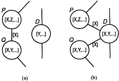
Steal-an-Edge. The Steal-an-Edge transformation is illustrated in Figure 2. An edge connecting two clusters P and Q is replaced by two edges which pass through a third cluster D. In order to retain the path property, variables carried by the edge {P, Q) are added to D if they are not already present. Note that the new edges { P,D) and (P, Q) need only carry the old separator of {P, Q), even if there is a larger inter­ section between D and the other clusters, as there is between D and Q in this example-if the path prop­ erty held before this transformation, then there must be some other path carrying Y between D and Q, and that path still exists after the transformation.

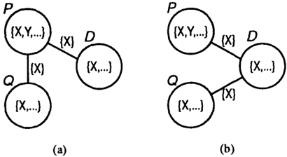
Slide and Drop. The Slide and Drop transforma­ tions can be seen as special cases of the Steal-an-Edge transformation where respectively one or both of the edges ( P,D} and { Q,D) already exist. An example of Slide is shown in Figure 3; it is so-named because it resembles sliding one end of an edge from one cluster to a neighboring cluster. A Drop transformation oc­ curs when there is a triangle, and one of its edges is simply deleted. In both cases, the "opposite" cluster (D) and the two edges to that cluster are augmented as necessary to carry the separator of the deleted edge.

Collapse. The Collapse transformation takes a sim­ ple cycle of clusters, deletes one edge from the cycle,

and restores the path property by added the separator of the deleted edge to each other cluster and edge in the cycle. Following the argument of [Shachter et a/., 1994], this is the transformational equivalent of Loop­ Cutset Conditioning.

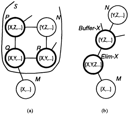
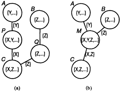
Node Elimination. Eliminating a node can be mod­ eled very elegantly as a transformation. The original definition of node elimination is: "select some vari­ able (i.e. node) X, add fill-arcs as necessary to connect all its un-eliminated neighbors, and mark X as elimi­ nated." Our Eliminate transformation takes as argu­ ments the variable X and a set of clusters S from which X is to be eliminated (here S typically corresponds to the clusters containing unmarked variables). Since our clusters represent cliques (or subsets of cliques) in the underlying graph, the set of (unmarked) neighbors of X is the union of all variables in all the clusters in S that contain X (the bold clusters in Figure 4(a)). Adding fill arcs to connect these neighbors is the same as merging those clusters in S that contain X into a single cluster ( Elim-X in Figure 4(b)). Marking the variable X as eliminated then translates to creating a second "buffer" cluster (Buffer·-X) which contains all of the variables of the elimination cluster except X, and which also inherits all the edges from other clusters in S that are incident to any of the merged clusters. By our construction, Elim-X is only connected to Buffer·­ X (within S), and cannot be part of any cycles re­ maining inS. Therefore Elim-X need not participate in any further transformations, and thus the variable X is effectively eliminated from consideration.

When a variable X is eliminated from a set S of clus­ ters, it is only eliminated from those clusters in S; there may be other clusters outside of S which still contain the variable X and are not merged into the elimination cluster (e.g. M in Figure 4). Thus in order to retain the path property, any edges from outside S to the merged clusters in S that carry X must be con­ nected to the elimination cluster rather than to the buffer cluster. (In fact, we simply migrate all edges between the merged clusters and clusters outside S to the elimination cluster.)

In Section 2 we indicated that it is not necessary to consider the entire cluster graph when doing transfor­ mations: we can restrict our attention to a biconnected component of the cluster graph. When the set S is a biconnected component, and a variable X is eliminated from S but remains present outside of S (as with X in M above), we have reproduced the refinement to the elimination algorithm described by [Kjrerulff, 1990, Theorem 3] (who further cites [Fujisawa and Orino, 1974] as its source). We wish to point out that this optimization arises quite naturally from the perspec­ tive of transformations and the need to preserve the path property.

Dropping Spurious Variables. Some transforma­ tions may result in a variable being present in a cluster where it serves no purpose: it is neither a member of

any family in that cluster, nor is it being carried from one cluster t.o another. We call such a variable a spu­ rious variable. (In order to detect spurious variables efficiently, we must note in each cluster which variables are part of families that must be preserved; obviously whenever clusters are merged, the new merged chls­ ter must inherit the 'family' annotations from the old clusters.) Figure 3 shows an example of how this could arise with a Slide transformation; if the variable X is present in P only so that P can carry X between Q and D, then after the transformation, X is spurious in P (and on the edge (P,D)). Spurious variables can be generated by all the above transformations except Steal-an-Edge.

Spurious variables are dropped by removing them from the pertinent cluster and from the (at most one) in­ cident edge that carries them. If either the edge or the cluster become empty as a result of this removal, they can be dropped from the cluster graph. We can either define the above transformations so they check for and remove spurious variables when they are cre­ ated, or spurious variable removal can be defined as a separate transformation in its own right (in which case the transformation should operate recursively, possibly removing entire chains of spurious variables).

A more general notion of spuriousness is possible. Con­ sider two clusters P and Q which need a variable X and are connected by two distinct. paths, both carry­ ing X. Unless every cluster on both of those paths also needs X, X could be removed from at least part of one of the paths without compromising the path property. A transformation which detected and removed X from some set of clusters and edges where it was not needed is possible, but the lack of locality of information might make it impractical.

For completeness, we will also describe the transfor­ mation corresponding to adding a single fill arc to the underlying moral graph of a belief network N. To add an arc from X toY, a cluster P that contains either X or Y is found. If cluster P already contains both of X and Y, then there is nothing more to be done. If not, the remaining variable (say Y) is added to P and the path property is restored by adding a new edge carrying Y from P to any other cluster containing Y.

There are a wide variety of possible cluster graph transformations. It seems likely that a successful gen­ eral clustering strategy would use only a few transfor­ mations, but there may also be transformations that are very useful in certain special cases.4

4 Algorithms

Now these transformations need to be put together into a sequence which will transform an arbitrary chls­ ter graph into a junction tree. The issue of termination must be addressed: it. should be clear that instances of the Slide transformation can undo each other, result­ ing in no progress. Cycles can also result from com­ binations of other transformations. We have not at­ tempted a general categorization of terminating trans­ formation sequences, but. we will characterize one class of algorithms that function by repeatedly identifying and transforming multiply-connected subgraphs of the cluster graph.

We will show that we can construct an algorithm to transform a cluster graph G into a junction tree start­ ing with any algorithm that can transform a multiply­ connected subgraph S of G into a singly-connected subgraph. The subgraph S is not required to include all the edges in G between clusters in S (see Fig­ ure 5(a)).

In Section 3, transformations were described as delet­ ing or adding edges to the graph. For the proof below, we will find it convenient to define rnigr·ating an edgf: to be deleting one edge and adding another with one of the same endpoints (e.g. deleting {A,B) and adding {A, C)). We also wish to generalize the idea of adding an edge so that we speak of "adding" an edge when the edge already exists in G, in which case the "new" edge is merged with the existing edge. For example, we will describe the Merge transformation as migrat­ ing edges, even when multiple edges become merged into one edge.

Theorem 2: An algorithm which functions by re­ peatedly finding some mult.iply-connected subgraph S of a cluster graph G (halting when there is no such S), and invoking a subroutine SUB on S, will termi­ nate with G transformed into a junction tree if the

4 An example is the "dynamic restructuring" transfor­ mation described in [Shachter et al., 1994], which can he used to take advantage of the location of evidence in junc­ tion trees of a certain topology.

subroutine SUB obeys these properties:

1. SUB terminates.
2. SUB uses only transformations which preserve the family and path properties with respect to t.he entire graph G.
3. SUB transforms S into a singly-connected sub­ graph.
4. The only effect SUB may have on clusters or edges outside of S is that:
5. (a) Edges not inS but between clusters inS may be deleted or migrated within S.
6. (b) Edges between clusters in G\S and clusters in S may be migrated, with only the endpoints inS permitted to move.

Proof: G is a junction tree if it is singly-connected and the family and path properties hold. That the family and path properties must always hold in G fol­ lows from property (2) above. To show that G must. become singly-connected, first. let us establish that it. cannot become disconnected by an invocation of SUB on a subgraph S. Clearly S cannot become discon­ nected, and any clusters in G that were connected by paths outside of S also remain connected. Let R be the set. of edges which connect dusters in G\S to dus­ ters in S. If there are two dusters P and Q in G\S that. were previously connected by some path pass­ ing through S, that path must have used some even number of edges from R. Suppose the first and last. of those edges were {Gl,Sl} and {S2, G2). After the subroutine, there must. still be two edges { Gl,Sx) and (Sy, G2} that are the possibly migrated versions of the old edges, and since S is connected, there must be a path from Sx to Sy, and thus between P and Q, and thus G remains connected. Now we will show that the quantity ( # edges in G) -( # clusters in G) must. de­ crease with each invocation of SUB; it must thus even­ tually reach -1, implying that G is singly-connected. This is a simple algebraic proof once we have defined several (}Uantities:

T G\ S = the dusters in G but not S befon: invoking SUB:

TIT 二

the number of dusters in

T

ns 二

the number of clusters in S

eT =

the number of edges between clusters in T

en 二

t.he number of edges between T and S

es =

the number of edges in S

ks es- ns 二

ex 三

the number of edges between clusters in S but not inS

after irwoking SUB:

D..s the change in ns =

the change in 6R =

e n

the change in ex 8x

Initially, the total number of clusters in G is ( nT + ns) and the number of edges is ( eT + eR + es +ex ). After SUB has been invoked, the number of clusters is ( nT + ns+.6.s) and the number of edges is ( eT+(eR+6R)+ (ns + .6-s1) +(ex + 6x )) . Putting all this together, we have:

Since ks ;=:: 0, and 6R, 6x � 0, the difference between the number of edges and the number of clusters in G must decrease by at least one with each invocation of SUB, and thus G must eventually become singly­ connected. D

Now we describe two algorithms for transforming an arbitrary cluster graph G into a junction tree. The first is the node elimination algorithm, and the second is a new algorithm.

4.1 Node Elimination

Given a set of clusters S, take the set of variables to be eliminated to be the union of the variables of each of the clusters in S. Choose some variable X to eliminate; when it has been eliminated, some subset of the clusters in S are merged, and two new clus­ ters, Elim-X and Buffer·-X, are created. Recursively call Node-Elimination on S\{Eiim-X}. Note that it is not necessary to continue until all variables have beeri eliminated, only until S is singly-connected.

If we let S be G in the original invocation of Node­ Elimination, this is the traditional node elimination algorithm. Alternatively, by Theorem 2, we could create a new algorithm by iteratively invoking Node­ Elimination on some other S.

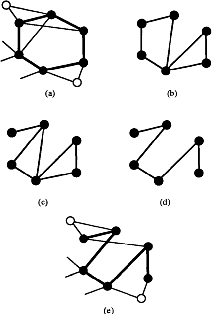
4.2 Divide Loops

Divide-Loops iteratively finds a cycle in the set of nodes and recursively "transforms it away" by a sub­ routine we will call Divide-a-Loop. Divide-a-Loop uses Steal-an-Edge or Slide to recursively subdivide a cy­ cle into smaller cycles (or into one smaller cycle and a "branch"), until eventually encountering cycles of length three, which are resolved by the Drop trans­ formation. Figure 5 shows an example. Theorem 2 guarantees that Divide-Loops will correctly transform G into a junction tree, since Divide-a-Loop clearly ter­ minates, and also cannot affect edges or clusters out­ side the cycle S on which it is invoked, except pos­ sibly to delete some other edges between clusters in S. Divide-Loops can be parameterized by the choice of which cycle to work on next, and Divide-a-Loop by

(e)

Figure 5: Divide-Loops transforms a graph into a tree by recursively subdividing each cycle.

which transformation to apply to which trio of clus­ ters. We have t.ried several greedy heuristics, discussed in Section 6.

4.3 Pre- and Postprocessing

In addition to procedures which render a subgraph S singly-connected, we may also consider procedures on S which transform it in other ways. Pr·epmassing is not aimed at making the subgraph singly-connected, but rather at simplifying it in ways we hope will im­ prove the performance of the main algorithm (either by making it faster, or by causing it to generate a lower cost tree). Postproassing takes a singly-connected subgraph and applies transformations to improve its cost. Pre- and postprocessing procedures can be ap­ plied globally to G or individually to subgraphs S.

Free-Variable-Elimination is a preprocessing proce­ dure which uses the Eliminate transformation to elim­ inate any variable that occurs in only one cluster in S. In node elimination, it. is known that free variables can always be eliminated first without increasing the cost of the final junction tree [Rose et a/., 1976].

Merging redundant clusters (where one cluster is a sub­ set of another) can be a preprocessing step. There is

one subtlety: suppose that P is a subset of Q, but some variables present in P are only in Q because Q is car­ rying them between two other neighbors (i.e. they are not part of any family in Q). It might be disadvanta­ geous to merge P and Q as a preprocessing step, be­ cause subsequent transformations might remove those variables from Q, if they are not merged. To avoid this, we require that the family variables of P be a subset of the family variables of Q.

Merging redundant dusters is also valuable as a post­ processing step. The definition of a junction tree given in Section 2 does not require that clusters must be cliques (that is, maximal), but clearly there is no ad­ vantage to retaining dusters which are not cliques.

In Section 3 (and Figure 3), we indicated that the Slide transformation might result in spurious variables, which could then be dropped. The combination of Slide and dropping spurious variables changes the cost of the cluster graph: the change is equal to the de­ crease in the size of the potential of the cluster which looses the edge (P in Figure 3) minus the increase in the size of the cluster which acquires the edge (D). Note that when Slide is applied to a tree, the result is also a tree. Thus we have the postprocessing procedure Slide-Beneficially, which "juggles" the edges oft.he tree about, finding Slide transformations which reduce the cost of the tree by dropping spurious variables.

5 Incremental Clustering

If the structure of a belief network is modified dynam­ ically, there are at least two reasons why it might be desirable to modify an existing junction tree incremen­ tally rather than generating a new one from scratch: (1) If the network is very large, modifying an exist­ ing junction tree might be considerably less expensive than generating a new one. (2) Incremental modifica­ tion should produce more stable results ( i. f. more like the previous tree), which is important. if the junction tree is being used by the network designer (especially if the designer is trying to optimize the junction tree itself).

Incremental clustering is very natural in our frame­ work. We assume that the basic acts in modifying the belief network are the addition or deletion of an arc or a variable.

To add a new variab/t;, Create a new cluster containing the variable (if the variable has parents, add ares as follows).

To add a new arc X-->Y. Find the cluster P containing the family of the variable Y, and add X to P and to the family. Find the cluster Q containing the family of X, and if it is not the same as P, add an edge (P,Q), or add X to the separator of the existing edge.

To delete an ar·c X-+ Y. Find the cluster P containing the family of the variable Y, and remove X from the family of Y. If X has become spurious in P, it may simply be dropped from P. If X does not appear in any other family in P, but still is not spurious in P (because P carries X between more than one other ad­ jacent clusters), we may retract X from P by adding edges (carrying X) sufficient to connect all of P's neigh­ bors which contain X, and removing X from P and all its incident edges. Retraction may be carried out re­ cursively until the only edges carrying X are between clusters which have X as a member of some family.5

To delete a var·iable. Delete all the arcs between the variable and all other variables, then remove the fam­ ily from its duster (and the duster itself, if it is now empty.)

If the modifications to the junction tree cause it to become multiply-connected, invoke some algorithm to transform it back into a tree. As with the transforma­ t.ions in Section 3, the correctness of these procedures follows from their maintenance of the family and path properties.

Incremental clustering might also be used when the network is modified in other ways. For example, a junction tree might be modified to optimize computa­ tion given the placement of evidence in the network. Or, if a particular query variable is identified, the junc­ tion tree could be modified to omit d-separated parts of the network.

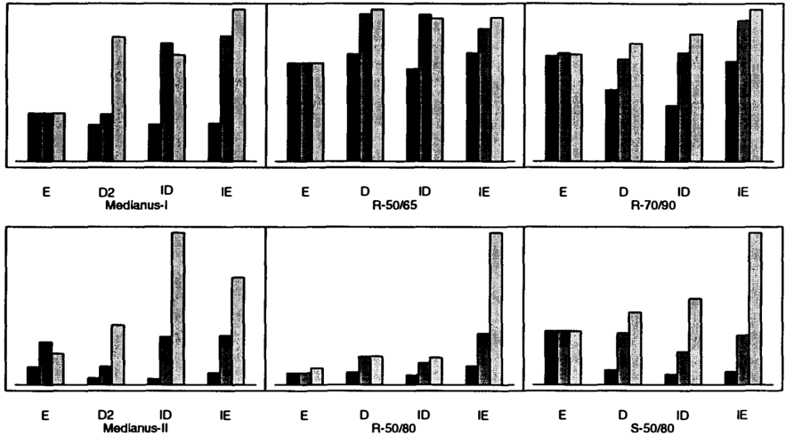
6 Some Empirical Results

The transformations from Section 3 and the algorithms from Section 4 have been implemented in Common Lisp. We have run experiments on two networks, the Medianus-1 and Medianus-11 networks used for the study of triangulation techniques in [Kjrerulff, 1990], and on four randomly generated networks. Medianus-1 has 43 variables and 66 arcs, Medianus-11 has 58 vari­ ables and 79 arcs, and the names of the randomly gen­ erated networks (see Figure 6) indicate their number of variables and arcs respectively. All the networks have non-binary variables. We performed two kinds of tests: "whole" tests, in which an algorithm was applied to an entire network (actually, to the bicon­ nected components of the original cluster graph), and ineremental tests where the network was built up (con­ tiguously) by adding arcs one by one, and calling one of the transformation algorithms whenever the cluster graph became multiply-connected. (We have not yet. experimented with retraetion.) For each kind of test, we ran the algorithms several times, randomly break­ ing any ties (e.g. generated by the heuristic ranking of whic.h transformation to perform next.).

For Node-Elimination we used the min-weight heuris-

5To completely reverse the operations which generated a junction tree, it is also necessary to be able to "take apart" clusters into their component families {connected by sufficient edges to guarantee the path property, naturally). Whether or when to do this would be a matter of heuristics.

tic, and Merge-Redundant-Clusters as a postprocess­ ing step (we also tried Slide-Beneficially, but it never helped). Quite a number of parameterizat.ions of Divide-Loops are possible: choices of which preor postprocessing steps to apply (and whether to apply them to each cycle individually, i. c. with each call to Divide-a-Loop, or to apply them to the entire graph), which cycle to work on next (we picked a cluster at ran­ dom, and tried finding the cycle according to shortest length, lowest cost, or a weighted combination of short­ est length and lowest cost), and which transformation to use to divide a cycle (minimize increase in any clus­ ter cost, minimize increase in overall cost, minimize increase in cluster degree, and combinations thereof). The results in Figure 6 show three different parame­ terizations of Divide-Loops (indicated by D, D2 and ID), which performed best, respectively, on "whole" experiments on the real networks, the "whole" exper­ iments on the artificial networks, and the incremental experiments on all networks.

D. Preprocessing: free variable elimination on each call to Divide-a-Loop. Choice of cycle: weighted com­ bination of shortest and cheapest (prefers shortest un­ less its very expensive). Choice of next transformation: minimize the increase in cluster cost. Postprocess the entire graph when finished by Slide-Beneficially fol­ lowed by Merge-Redundant-Clusters.

D2. The same as D, except that choice of cycle is shortest cycle.

ID. The same as D, except that t.he postprocessing is done on each call to Divide-a-Loop, and does not include merging.

Probably the most surprising result was that merging redundant clusters is a very bad idea, except after all other processing has been done (and since there is no "last" in incremental clustering, it is best not to do it at all; but the results seem to show that this does not significantly affect the cost of the result).

The strongest impression from our "whole" experi­ ments is that. Divide-Loops has high variance, no mat­ ter what choice of parameters is used. In some cases the median may be lower than node elimination, but the average is always higher (but also, the minimum can be much lower). Since Divide-Loops works on only a single cycle at a time, it is perhaps not surprising that its performance is substantially the same when applied incrementally as when applied "whole" (ex­ cept for Medianus-11). Node-Elimination, on the other hand, performs generally worse when applied incre­ mentally, especially on the denser networks. It also appears that Divide-Loops competes more favorably with Node-Elimination on the denser networks than on the sparser networks.

Overall, these results indicate that while we have not found an algorithm which is superior to Node­ Elimination, we have found a new algorithm, based on different principles, which is comparable. This en­ courages us to believe that our clustering framework

may yield other good algorithms in the future.

7 Conclusion

Not long after beginning this research, we implemented a simple graphical interface to demonstrate the ef­ fect of some transformations. With this interface, we quickly discovered the existence of spurious variables, and were able to rule out some heuristics as ineffec­ tive. The graphical interface, and the simple visual nature of the transformations, greatly aided our un­ derstanding. We feel that this simplicity should be equally beneficial to belief network designers, making it easier to understand the computational properties of networks.

Further, viewing clustering as a process of transforma­ tions opens up a wide vista of possible new heuristic approaches to clustering, some of which may prove superior to known methods. However there are so many possible transformations and algorithms to em­ ploy them that we have something of an embarrass­ ment of riches-there are simply too many possibili­ ties to explore. Analysis revealing some organizational properties of this space would be quite helpful-for ex­ ample, what sets of transformations are complete in the sense that they can generate all minimal triangu­ lations?

In summary, we have presented a new framework for clustering algorithms, based on transformations of a cluster graph rather than on triangulation. We have demonstrated a set of transformations within this framework, and presented a new algorithm based on those transformations. We have also demonstrated an algorithm for incrementally clustering a dynamically changing network.

Acknowledgments

We thank Uffe Kjrerulff for providing us with the Medianus-I and Medianus-11 networks, and Mike Williamson for insightful comments on the paper. This research was funded by National Science Foundation Grant IRI-9008670.

References

• [Almond and Kong, 1991] Russell Almond and Au­ gustine Kong. Optimality issues in constructing a markov tree from graphical models. Research Re­ port A-3, Harvard University, April 1991.
• [Arnborg et al., 1987] Stefan Arnborg, Derek G. Corneil, and Andrzej Proskurowski. Complexity of finding embeddings in a k-tree. SIAM .lour·nal on Algebraic and Discrdt: Mdhods, 8(2):277-284, April 1987.
• [Fujisawa and Orino, 1974] T. Fujisawa and H. Orino. An efficient algorithm of finding a minimal triangu-
• lation of a graph. In IEEE Inter-national Symposium on Circuit!.i and Systems, pages 172-175, 1974.
• [Jensen and Jensen, 1994] Finn V. Jensen and Frank Jensen. Optimal junction trees. In Pr·oceedings UAI94, pages 360-366, Seattle, WA, July 1994.
• [Jensen et al., 1990a] Finn V. Jensen, Steffen L. Lau­ ritzen, and K. G. Olesen. Bayesian updating in causal probabilistic networks by local computa­ tions. Computational Statistics Quartt:r-ly, 4:269282, 1990.
• [Jensen et al., 1990b] Finn V. Jensen, K. G. Olesen, and S. K. Anderson. An algebra of Bayesian belief universes for knowledge-based systems. Ndworks, 20(5):637-59, 1990.
• [Jensen, 1988] Finn V. Jensen. Junction trees and de­ composable hypergraphs. Research report, Judex Datasystemer, Aalborg, Denmark, 1988.
• [Kjrerulff, 1990] Uffe Kjrerulff. Triangulation of graphs-algorithms giving small total state space. Technical Report R 90-09, Department of Mathe­ matics and Computer Science, Aalborg University, Denmark, March 1990.
• [Lauritzen and Spiegelhalt.er, 1988] Steffen L. Lau­ ritzen and David J. Spiegelhalter. Local computa­ tions with propabilities on graphical structures and their application to expert systems. .lour·nal of tht: Royal Stati!.itical Society B, 50(2):157-224, 1988.
• [Pearl, 1988] Judea Pearl. Pr·obabilistic Rt:asoning in Intdlig.wt Systnns: N d w or· k s of Plausiblt: Inft:r·­ t:Tiet:. Morgan Kaufmann, San Mateo, California, 1988.
• [Rose et al. , 1976] Donald J. Rose, R. Endre Tarjan, and George S. Lenker. Algorithmic aspects of vertex elimination on graphs. SIAM Journal on Comput­ ing, 5(2):266-283, 1976.
• [Shachter d al. , 1994] Ross D. Shachter, Stig. K. An­ derson, and Peter Szolovits. Global conditioning for probabilistic inference in belief networks. In Pr-o­ at:dings UAI-94, pages 514-522, Seattle, WA, July 1994.