Combining Spatial and Temporal Logics: Expressiveness vs. Complexity

David Gabelaia Roman Kontchakov Agi Kurucz

[email protected] [email protected] [email protected]

Department of Computer Science, King's College London Strand, London WC2R 2LS, U.K.

Frank Wolter

[email protected]

Department of Computer Science, University of Liverpool Liverpool L69 7ZF, U.K.

Michael Zakharyaschev

[email protected]

Department of Computer Science, King's College London Strand, London WC2R 2LS, U.K.

Abstract

In this paper, we construct and investigate a hierarchy of spatio-temporal formalisms that result from various combinations of propositional spatial and temporal logics such as the propositional temporal logic PT L , the spatial logics RCC -8, BRCC -8, S 4 u and their fragments. The obtained results give a clear picture of the trade-off between expressiveness and 'computational realisability' within the hierarchy. We demonstrate how different combining principles as well as spatial and temporal primitives can produce NP-, PSPACE-, EXPSPACE-, 2EXPSPACE-complete, and even undecidable spatio-temporal logics out of components that are at most NP- or PSPACE-complete.

1. Introduction

Qualitative representation and reasoning has been quite successful in dealing with both time and space. There exists a wide spectrum of temporal logics (see, e.g., Allen, 1983; Clarke & Emerson, 1981; Manna & Pnueli, 1992; Gabbay, Hodkinson, & Reynolds, 1994; van Benthem, 1995). There is a variety of spatial formalisms (e.g., Clarke, 1981; Egenhofer & Franzosa, 1991; Randell, Cui, & Cohn, 1992; Asher & Vieu, 1995; Lemon & Pratt, 1998). In both cases determining the computational complexity of the respective reasoning problems has been one of the most important research issues. For example, Renz and Nebel (1999) analysed the complexity of RCC -8, a fragment of the region connection calculus RCC with eight jointly exhaustive and pairwise disjoint base relations between spatial regions introduced by Egenhofer and Franzosa (1991) and Randell and his colleagues (1992); Nebel and B¨ urckert (1995) investigated the complexity of Allen's interval algebra; numerous results on the computational complexity of the point-based propositional linear temporal logic PT L over various flows of time were obtained by Sistla and Clarke (1985) and Reynolds (2003, 2004). In many cases these investigations resulted in the development and implementation of effective reasoning algorithms (see, e.g., Wolper, 1985; Smith & Park, 1992; Egenhofer & Sharma, 1993; Schwendimann, 1998; Fisher, Dixon, & Peim, 2001; Renz & Nebel, 2001; Hustadt & Konev, 2003).

.

The next apparent and natural step is to combine these two kinds of reasoning. Of course, there have been attempts to construct spatio-temporal hybrids. For example, the intended interpretation of Clarke's (1981, 1985) region-based calculus was spatio-temporal. Region connection calculus RCC (Randell et al., 1992) contained a function space ( X,t ) for representing the space occupied by object X at moment of time t . Muller (1998a) developed a first-order theory for reasoning about motion of spatial entities. However, all of these formalisms turn out to be 'too expressive' from the computational point of view: they are undecidable . Moreover, as far as we know, no serious attempts to investigate and implement partial (say, incomplete) algorithms capable of spatio-temporal reasoning with these logics have been made.

The problem of constructing spatio-temporal logics with better algorithmic properties and analysing their computational complexity was first attacked by Wolter and Zakharyaschev (2000b); see also the 'popular' and extended version (Wolter & Zakharyaschev, 2002) of that conference paper, as well as (Bennett & Cohn, 1999; Bennett, Cohn, Wolter, & Zakharyschev, 2002; Gerevini & Nebel, 2002).

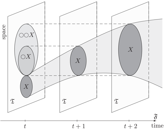
The main idea underlying all these papers is to consider various combinations of 'wellbehaved' spatial and temporal logics. The intended spatio-temporal structures can be regarded then as the Cartesian products of the intended time-line and topological (or some other) spaces that are used to model the spatial dimension. Figure 1 shows such a product (of the flow of time F = 〈 N , < 〉 and the two-dimensional Euclidean space T ) with a moving spatial object X . The moving object can be viewed either as a 3D spatio-temporal entity (in this particular case) or as the collection of the 'snapshots' or slices of this entity at each moment of time; for a discussion see, e.g., (Muller, 1998b) and references therein. In this paper, we use the snapshot terminology and understand by a moving spatial object (or, more precisely, interpret such an object as) any set of pairs 〈 X,t 〉 where, for each point t

.

of the flow of time, X is a subset of the topological space-the state of the spatial object at moment t .

The expressive power (and consequently the computational complexity) of the combined spatio-temporal formalisms obviously depends on three parameters:

1. the expressivity of the spatial component,
2. the expressivity of the temporal component, and
3. the interaction between the two components allowed in the combined logic.

Regardless of the chosen component languages, the minimal requirement for a spatiotemporal combination to be useful is its ability to

Typical examples of logics meeting this spatial propositions' truth change principle are the combinations of RCC -8 and Allen's interval calculus (Bennett et al., 2002; Gerevini & Nebel, 2002) and those combinations of RCC -8 and PT L introduced by Wolter and Zakharyaschev (2000b) that allow applications of temporal operators to Boolean combinations of RCC -8 relations. Languages satisfying (PC) can capture, for instance, some aspects of the continuity of change principle (see, e.g., Cohn, 1997) such as

• (A) if two images on the computer screen are disconnected now, then they either remain disconnected or become externally connected in one quantum of the computer's time.

Another example is the following statement about the geography of Europe:

• (B) Kaliningrad is disconnected from the EU until the moment when Poland becomes a tangential proper part of the EU, after which Kaliningrad and the EU will be externally connected forever.

However, languages meeting (PC) do not necessarily satisfy our second fundamental spatial object change principle according to which we should be able to

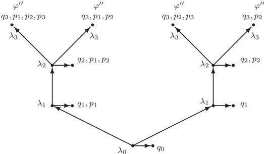
In logical terms, (PC) refers to the change of truth-values of propositions, while (OC) to the change of extensions of predicates; see Fig. 2 where © X at moment t denotes the state of X at moment t +1. Here are some examples motivating (OC):

• (C) Continuity of change: 'the cyclone's current position overlaps its position in an hour.'
• (D) Two physical objects cannot occupy the same space: 'if tomorrow object X is at the place where object Y is today, then Y will have to move by tomorrow.'
• (E) Geographic regions change: 'the space occupied by Europe never changes.'
• (F) Geographic regions change: 'in two years the EU will be extended with Romania and Bulgaria.'
• (G) Fairness conditions on regions: 'it will be raining over every part of England ever and ever again.'

.

• (H) Mutual exclusion: 'if Earth consists of water and land, and the space occupied by water expands, then the space occupied by land shrinks.'

It should be clear that to represent these statements we have to refer to the evolution of spatial objects in time (say, to compare objects X and ©© X )-it is not enough to only take into account the change of the truth-values of propositions speaking about spatial objects.

The main aim of this paper is to investigate the trade-off between the expressive power and the computational behaviour of spatio-temporal hybrids satisfying the (PC) and (OC) principles and interpreted in various spatio-temporal structures. Our purpose is to show what computational obstacles one can expect if the application domain requires this or that kind of interactions between temporal and spatial operators.

The spatio-temporal logics we consider below are combinations of fragments of PT L interpreted over different flows of time with fragments of the propositional spatial logic S 4 u (equipped with the interior and closure operators, the universal and existential quantifiers over points in space as well as the Booleans) interpreted in topological spaces. This choice is motivated by the following reasons:

• The component logics are well understood and established in temporal and spatial knowledge representation; all of them are supported by reasonably effective reasoning procedures.
• By definition, implicit or explicit temporal quantification is necessary to capture (OC), and fragments of PT L are the weakest languages with such quantification we know of.

Allen's interval calculus, for example, does not provide means for any quantification over intervals. It is certainly suitable for spatio-temporal hybrids satisfying (PC) (see Bennett et al., 2002; Gerevini & Nebel, 2002) but there is no natural conservative way of combining it with spatial formalisms to meet (OC). On the other hand, it is embedded in PT L (Blackburn, 1992). A natural alternative to PT L would be the extension of Allen's calculus by means of quantification over intervals introduced by Halpern and Shoham (1986), but unfortunately this temporal logic turns out to be highly undecidable.

• Although the logic S 4 u was originally introduced in the realm of modal logic (see below for details), the work of Bennett (1994), Nutt (1999), Renz (2002) and Wolter and Zakharyaschev (2000a) showed that it can be regarded as a unifying language that contains many spatial formalisms like RCC -8, BRCC -8 or the 9-intersections of Egenhofer and Herring (1991) as fragments.

Apart from the choice of component languages and the level of their interaction, the expressive power and the computational complexity of spatio-temporal logics strongly depend on the restrictions we may want to impose on the intended spatio-temporal structures and the interpretations of spatial objects.

• We can choose among different flows of time (say, discrete or dense, infinite or finite)
• and among different topological spaces (say, arbitrary, Euclidean or Aleksandrov).
• At each time point we can interpret spatial objects as arbitrary subsets of the topological space, as regular closed (or open) ones, as polygons, etc.
• To represent the assumption that everything eventually comes to an end, we only do not know when, one can restrict the class of intended models by imposing the finite change assumption which states that no spatial object can change its spatial configuration infinitely often, or the more 'liberal' finite state assumption according to which every spatial object can have only finitely many possible states (although it may change its states infinitely often).

The paper is organised as follows. In Section 2 we introduce in full detail the component spatial and temporal logics to be combined later on. In particular, besides the standard spatial logics like RCC -8 or the 9-intersections of Egenhofer and Herring (1991), we consider their generalisations in the framework of S 4 u and investigate the computational complexity. For example, we show that the maximal fragment of S 4 u dealing with regular closed spatial objects turns out to be PSPACE-complete, while a natural generalisation of the 9-intersections is still in NP. In Section 3 we introduce a hierarchy of spatio-temporal logics outlined above, provide them with a topological-temporal semantics, and analyse their computational properties. First we show that spatio-temporal logics satisfying only the (PC) principle are not more complex than their components. Then we consider 'maximal' combinations of S 4 u with (fragments of) PT L meeting both (PC) and (OC) and see that this straightforward approach does not work: the resulting logics turn out to be undecidable. Finally, we systematically investigate the trade-off between expressivity and complexity of spatio-temporal formalisms and construct a hierarchy of decidable logics satisfying (PC)

and (OC) whose complexity ranges from PSPACE to 2EXPSPACE. These and other results, possible implementations as well as open problems are discussed in Section 4. For the reader's convenience most important (un)decidability and complexity results obtained in this paper are summarised in Table 1 on page 193. All technical definitions and detailed proofs can be found in the appendices.

2. Propositional Logics of Space and Time

We begin by introducing and discussing the spatial and the temporal formalisms we are going to combine later on in this paper.

2.1 Logics of Space

We will be dealing with a number of logics suitable for qualitative spatial representation and reasoning: the well-known RCC -8, BRCC -8 and S 4 u , as well as certain fragments of the last one. The intended interpretations for all of these logics are topological spaces.

A topological space is a pair T = 〈 U, I 〉 in which U is a nonempty set, the universe of the space, and I is the interior operator on U satisfying the standard Kuratowski axioms : for all X,Y ⊆ U ,

The operator dual to I is called the closure operator and denoted by C : for every X ⊆ U , we have C X = U -I ( U -X ). Thus, I X is the interior of a set X , while C X is its closure . X is called open if X = I X and closed if X = C X . The complement of an open set is closed and vice versa. The boundary of a set X ⊆ U is defined as C X -I X . Note that X and U -X have the same boundary.

2.1.1 S 4 u

Our most expressive spatial formalism is S 4 u -i.e., the propositional modal logic S 4 extended with the universal modalities. The 'pedigree' of this logic is quite unusual. S 4 was introduced independently by Orlov (1928), Lewis (in Lewis & Langford, 1932), and G¨ odel (1933) without any intention to reason about space. Orlov and G¨ odel understood it as a logic of 'provability' (in order to provide a classical interpretation for the intuitionistic logic of Brouwer and Heyting) and Lewis as a logic of necessity and possibility, that is, as a modal logic . Besides the Boolean connectives and propositional variables, the language of S 4 contains two modal operators: I (it is necessary or provable) and C , the dual of I (it is possible or consistent). In other words, the formulas of S 4 can be defined as follows:

where the p are variables. Set C τ = I τ . We denote the modal operators by I and C (rather than the conventional ✷ and ✸ ) because we understand, following an observation made by several logicians in the late thirties and early forties (Stone, 1937; Tarski, 1938; Tsao Chen, 1938; McKinsey, 1941), S 4 as a logic of topological spaces : if we interpret the propositional variables as subsets of a topological space, the Booleans as the standard settheoretic operations, and I and C as, respectively, the interior and the closure operators

on the space, then an S 4-formula is modally consistent if and only if it is satisfiable in a topological space-i.e., its value is not empty under some interpretation. 1

More precisely, a topological model is a pair of the form M = 〈 T , U 〉 , where T = 〈 U, I 〉 is a topological space and U , a valuation , is a map associating with every variable p a set U ( p ) ⊆ U . Then the valuation U is inductively extended to arbitrary S 4-formulas by taking:

Expressions τ of the form (1) are interpreted as subsets of topological spaces; that is why we will call them spatial terms . In particular, propositional variables of S 4 will be understood as spatial variables .

The language of S 4 u extends S 4 with the universal and the existential quantifiers ✷ ∀ and ✸ ∃ , respectively (known in modal logic as the universal modalities ). Given a spatial term τ , we write ✸ ∃ τ to say that the part of space (represented by) τ is not empty (there is at least one point in τ ); ✷ ∀ τ means that τ occupies the whole space (all points belong to τ ). By taking Boolean combinations of such expressions we arrive at what will be called spatial formulas . A BNF definition looks as follows: 2

where the τ are spatial terms. Set ✸ ∃ τ = ¬ ✷ ∀ τ . Spatial formulas can be either true or false in topological models. The truth-relation M | = ϕ -a spatial formula ϕ is true in a topological model M -is defined in the standard way:

• M | = ✷ ∀ τ iff U ( τ ) = U ,
• M | = ¬ ϕ iff M /negationslash| = ϕ ,
• M | = ϕ 1 ∧ ϕ 2 iff M | = ϕ 1 and M | = ϕ 2 .

Say that a spatial formula ϕ is satisfiable if there is a topological model M such that M | = ϕ .

The seemingly simple 'query language' S 4 u can express rather complex relations between sets in topological spaces. For example, the formula

says that a set q is dense in a nonempty set p , but has no interior (here τ 1 /squareimage τ 2 is an abbreviation for τ 1 /intersectionsq τ 2 ).

The following 'folklore' complexity result has been proved in different settings (see, e.g., Nutt, 1999; Areces, Blackburn, & Marx, 2000):

Theorem 2.1. (i) S 4 u enjoys the exponential finite model property; i.e., every satisfiable spatial formula ϕ is satisfiable in a topological space whose size is at most exponential in the size of ϕ .

• (ii) Satisfiability of spatial formulas in topological models is PSPACE -complete.

1. Moreover, according to McKinsey (1941) and McKinsey and Tarski (1944), any n -dimensional Euclidean space, for n ≥ 1, is enough to satisfy all consistent S 4-formulas.

2. Formally, the language of S 4 u as defined above is weaker than the standard one, say, that of Goranko and Passy (1992). However, one can easily show that they have precisely the same expressive power: see, e.g., (Hughes & Cresswell, 1996) or (Aiello & van Benthem, 2002b).

One way of proving this theorem is first to observe that every satisfiable spatial formula is satisfied in an Aleksandrov model , i.e., a model based on an Aleksandrov topological space-alias a standard Kripke frame for S 4 (see, e.g., McKinsey & Tarski, 1944; Goranko & Passy, 1992).

We remind the reader that a topological space is called an Aleksandrov space (Alexandroff, 1937) if arbitrary (not only finite) intersections of open sets are open. A Kripke frame (or simply a frame ) for S 4 is a pair the form G = 〈 V, R 〉 , where V is a nonempty set and R a transitive and reflexive relation (i.e., a quasi-order ) on V . Every such frame G induces the interior operator I G on V : for every X ⊆ V ,

In other words, the open sets of the topological space T G = 〈 V, I G 〉 are the upward closed (or R -closed ) subsets of V . The minimal neighbourhood of a point x in T G (that is the minimal open set to contain x ) consists of all those points that are R -accessible from x . It is well-known (see, e.g., Bourbaki, 1966) that T G is an Aleksandrov space and, conversely, every Aleksandrov space is induced by a quasi-order.

Now, to complete the proof, it suffices to recall that S 4 is PSPACE-hard (Ladner, 1977) and use, say, the standard tableau technique to establish the exponential finite model property and construct a PSPACE satisfiability checking algorithm for spatial formulas.

Although being of the same computational complexity as S 4, the logic S 4 u is more expressive. A standard example is that spatial formulas can distinguish between arbitrary and connected 3 topological spaces. Consider, for instance, the formula

saying that p is both closed and open, nonempty and does not coincide with the whole space. It can be satisfied only in a model whose underlying topological space is not connected, while all satisfiable S 4-formulas are satisfied in connected (e.g., Euclidean) spaces.

Another example illustrating the expressive power of S 4 u is the formula

defining a nonempty set p such that both p and p have empty interiors. In fact, the second and the third conjuncts say that p and p consist of boundary points only.

2.1.2 RCC -8 as a Fragment of S 4 u

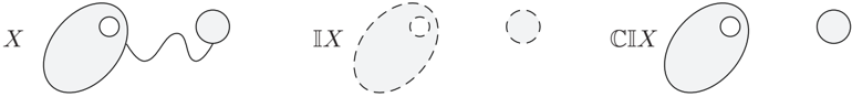
In qualitative spatial representation and reasoning, it is quite often assumed that spatial terms can only be interpreted by regular closed (or open) sets of topological spaces (see, e.g., Davis, 1990; Asher & Vieu, 1995; Gotts, 1996). One of the reasons for imposing this restriction is to exclude from consideration such 'pathological' sets as p in (3). Recall that a set X is regular closed if X = CI X , which clearly does not hold for any set p satisfying (3). Another reason is to ensure that the space occupied by a physical body is homogeneous in the sense that it does not contain parts of 'different dimensionality.' For example, the

3. We remind the reader that a topological space is connected if its universe cannot be represented as the union of two disjoint nonempty open sets.

.

subset X of the Euclidean plane in Fig. 3 consists of three parts: a 2D ellipse with a hole, a 2D circle, and a 1D curve connecting them. This curve disappears if we form the set CI X , which is regular closed because CICI X = CI X , for every X and every topological space.

In this paper, we will consider several fragments of S 4 u dealing with regular closed sets . From now on we will call such sets regions . Perhaps, the best known language devised for speaking about regions is RCC -8 which was introduced in the area of Geographical Information Systems (see Egenhofer & Franzosa, 1991; Smith & Park, 1992) and as a decidable subset of Region Connection Calculus RCC (Randell et al., 1992). The syntax of RCC -8 contains eight binary predicates,

• DC ( X,Y ) - regions X and Y are disconnected,
• EC ( X,Y ) -X and Y are externally connected,
• EQ ( X,Y ) -X and Y are equal,
• PO ( X,Y ) -X and Y partially overlap,
• TPP ( X,Y ) -X is a tangential proper part of Y ,
• NTPP ( X,Y ) -X is a nontangential proper part of Y ,
• the inverses of the last twoTPPi ( X,Y ) and NTPPi ( X,Y ),

which can be combined using the Boolean connectives. For example, given a spatial database describing the geography of Europe, we can query whether the United Kingdom and the Republic of Ireland share a common border. The answer can be found by checking whether the RCC -8 formula EC ( UK , RoI ) follows from the database.

The arguments of the RCC -8 predicates are called region variables ; they are interpreted by regular closed sets-i.e., regions-of topological spaces. The satisfiability problem for RCC -8 formulas under such interpretations is NP-complete (Renz & Nebel, 1999).

The expressive power of RCC -8 is rather limited. It only operates with 'simple' regions and does not distinguish between connected and disconnected ones, regions with and without holes, etc. (Egenhofer & Herring, 1991). Nor can RCC -8 represent complex relations between more than two regions. Consider, for example, three countries (say, Russia, Lithuania and Poland) such that not only each one of them is adjacent to the others, but there is a point where all the three meet. To express this fact we may need a ternary predicate like

To analyse possible ways of extending the expressive power of RCC -8, it will be convenient to view it as a fragment of S 4 u (that RCC -8 can be embedded into S 4 u was first shown by Bennett, 1994). Observe first that, for every spatial variable p , the spatial term

is interpreted as a regular closed set in every topological model. So, with every region variable X of RCC -8 we can associate the spatial term /rho1 X = CI p X , where p X is a spatial variable, and then translate the RCC -8 predicates into spatial formulas by taking:

( TPPi and NTPPi are the mirror images of TPP and NTPP , respectively). The first of these formulas, for instance, says that two regions are externally connected iff the intersection of the regions is not empty, whereas the intersection of their interiors is. It should be clear that an RCC -8 formula is satisfiable in a topological space if and only if its translation into S 4 u defined above is satisfiable in a topological model.

This translation also shows that in RCC -8 any two regions can be related in terms of truth/falsity of atomic spatial formulas of the form

where /rho1 1 and /rho1 2 are spatial terms of the form (5). For example, the first of these formulas says that the intersection of two regions is empty, whereas the last one states that one region is contained in the interior of another one. In other words, RCC -8 can be regarded as part of the following fragment of S 4 u :

Here we distinguish between two types of spatial terms. Those of the form /rho1 will be called atomic region terms -they represent the (regular closed) regions we want to compare. Spatial terms of the form τ are used to relate regions to each other (note that their extensions are not necessarily regular closed).

Actually, the fragment introduced above is a bit more expressive than RCC -8: for example, it contains (appropriately modified) formula (2) which can be satisfied only in disconnected topological spaces, while all satisfiable RCC -8 formulas are satisfiable in any Euclidean space (Renz, 1998). However, it will be convenient for us not to distinguish between these two spatial logics. First, it will turn out that the same technical results regarding their computational complexity hold for them even when combined with temporal

logics. And second, the more intuitive and concise language of RCC -8 is more suitable for illustrations. For instance, we do not distinguish between the region variable X and the region term /rho1 X and use DC ( /rho1 1 , /rho1 2 ) as an abbreviation for ¬ ✸ ∃ ( /rho1 1 /intersectionsq /rho1 2 ).

The definition above suggests two ways of increasing the expressive power of RCC -8 (while keeping all regions regular closed):

• (i) by allowing more complex region terms /rho1 , and
• (ii) by allowing more ways of relating them (i.e., more complex terms τ ).

2.1.3 BRCC -8 as a Fragment of S 4 u

The language BRCC -8 of Wolter and Zakharyaschev (2000a) (see also Balbiani, Tinchev, & Vakarelov, 2004) extends RCC -8 in direction (i). It uses the same eight binary predicates as RCC -8 and allows not only atomic regions but also their intersections, unions and complements. For instance, in BRCC -8 we can express the fact that a region (say, the Swiss Alps) is the intersection of two other regions (Switzerland and the Alps in this case):

We can embed BRCC -8 to S 4 u by using almost the same translation as in the case of RCC -8. The only difference is that now, since Boolean combinations of regular closed sets are not necessarily regular closed, we should prefix compound spatial terms with CI . This way we can obtain, for example, the spatial term

representing the Swiss Alps. In the same manner we can treat other set-theoretic operations, which leads us to the following definition of Boolean region terms :

In other words, Boolean region terms denote precisely the members of the well-known Boolean algebra of regular closed sets. (The union /unionsq is expressible via intersection and complement in the usual way.) To simplify notation, given a spatial term τ , we write ⌈ τ ⌉ to denote the result of prefixing CI to every subterm of τ ; in particular,

Note that ⌈ τ ⌉ is (equivalent to) a Boolean region term, for every spatial term τ . Now the Swiss Alps from the example above can be represented as ⌈ Switzerland /intersectionsq Alps ⌉ .

It is of interest to note that Boolean region terms do not increase the complexity of reasoning in arbitrary topological models: the satisfiability problem for BRCC -8 formulas is still NP-complete (however, it becomes PSPACE-complete if all intended models are based on connected spaces). On the other hand, BRCC -8 allows some restricted comparisons of more than two regions as, e.g., in (6). Nevertheless, as we shall see below, ternary relations like (4) are still unavailable in BRCC -8: they require different ways of comparing regions; cf. (ii).

2.1.4 RC

Egenhofer and Herring (1991) proposed to relate any two regions in terms of the 9-intersections-3 × 3-matrix specifying emptiness/nonemptiness of all (nine) possible intersections of the interiors, boundaries and exteriors of the regions. Recall that, for a region X , these three disjoint parts of the space 〈 U, I 〉 can be represented as

respectively. By generalising this approach to any finite number of regions, we obtain the following fragment RC of S 4 u :

In other words, in RC we can define relations between regions in terms of emptiness/nonemptiness of sets formed by using arbitrary set-theoretic operations on regions and their interiors. However, nested applications of the topological operators are not allowed (an example where such applications are required can be found in the next section).

Clearly, both RCC -8 and BRCC -8 are fragments of RC . Moreover, unlike BRCC -8, the language of RC allows us to consider more complex relations between regions. For instance, the ternary relation required in (4) can now be defined as follows:

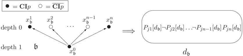
Another, more abstract, example is the formula

which says that regions /rho1 1 , . . . , /rho1 i meet somewhere inside the region occupied jointly by all /rho1 i +1 , . . . , /rho1 j , but outside the regions /rho1 j +1 , . . . , /rho1 k and not inside /rho1 k +1 , . . . , /rho1 n .

Although RC is more expressive than both RCC -8 and BRCC -8, reasoning in this language is still of the same computational complexity:

Theorem 2.2. The satisfiability problem for RC -formulas in arbitrary topological models is NP -complete.

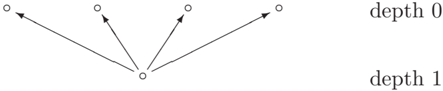
This result will be proved in Appendix A. Lemma A.1 shows that every satisfiable RC -formula can be satisfied in a model based on the Aleksandrov space that is induced by a disjoint union of n -brooms -i.e., quasi-orders of the form depicted in Fig. 4. Topological spaces of this kind have a rather primitive structure satisfying the following property:

• (rc) only the roots of n -brooms can be boundary points, and the minimal neighbourhood of every boundary point-i.e., the n -broom containing this point-must contain at least one internal point and at least one external point.

❜

❜

❜

❜

❜

For example, spatial formula (3) cannot be satisfied in a model with this property, and so it is not in RC .

By Lemma A.2, the size of such a satisfying model is polynomial (in fact, quadratical) in the length of the input RC -formula, and so we have a nondeterministic polynomial time algorithm. Actually, the proof is a straightforward generalisation of the complexity proof for BRCC -8 given by Wolter and Zakharyaschev (2000a): the only difference is that in the case of BRCC -8 it is sufficient to consider only 2-brooms (which were called forks ). This means, in particular, that ternary relation (4)-which is satisfiable only in a model with an n -broom, for n ≥ 3-is indeed not expressible in BRCC -8.

Remark 2.3 . In topological terms, n -brooms are examples of so-called door spaces where every subset is either open or closed. However, the modal theory of n -brooms defines a wider and more interesting topological class known as submaximal spaces in which every dense subset is open. Submaximal spaces have been around since the early 1960s and have generated interesting and challenging problems in topology. For a survey and a systematic study of these spaces see (Arhangel'skii & Collins, 1995) and references therein.

2.1.5 RC max

One could go even further in direction (ii) and impose no restrictions whatsoever on the ways of relating Boolean region terms. This leads us to the maximal fragment RC max of S 4 u in which spatial terms are interpreted by regular closed sets. Its syntax is defined as follows:

To understand the difference between RC and RC max , consider the RC max -formula

The price we have to pay for this expressivity is that the complexity of RC max is the same as that of full S 4 u :

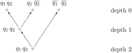
It says that the boundary of ⌈ q 1 ⌉ is not empty and that every neighbourhood of every point in this boundary contains an internal point of ⌈ q 1 ⌉ that belongs to the boundary of ⌈ q 2 ⌉ (compare with property (rc) above). The simplest Aleksandrov model satisfying this formula is of depth 2; it is shown in Fig. 5.

❜

Figure 5: Model satisfying formula (7).

Theorem 2.4. The satisfiability problem for RC max -formulas is PSPACE -complete.

The upper bound follows from Theorem 2.1 and the lower bound is proved in Appendix A, where we construct a sequence of RC max -formulas such that each of them is satisfiable in an Aleksandrov space of cardinality at least exponential in the length of the formula. The first formula of the sequence is similar to (7) above.

It is of interest to note, however, that RC max is still not expressive enough to define such 'pathological' sets as p in (3) which is clearly not regular closed.

To conclude this section, we summarise the inclusions between the spatial languages introduced above:

For more discussions of spatial logics of this kind we refer the reader to the paper (PrattHartmann, 2002).

2.2 Temporal Logics

As was said in the introduction, the temporal components of our spatio-temporal hybrids are (fragments of) the propositional temporal logic PT L interpreted in various flows of time which are modelled by strict linear orders F = 〈 W,< 〉 , where W is a nonempty set of time points and < is a (connected, transitive and irreflexive) precedence relation on W .

The language PT L is based on the following alphabet:

• propositional variables p 0 , p 1 , . . . ,
• the Booleans ¬ and ∧ , and
• the binary temporal operators U ('until') and S ('since').

The set of PT L -formulas is defined in the standard way:

PT L -models are pairs of the form M = 〈 F , V 〉 such that F = 〈 W,< 〉 is a flow of time and V , a valuation , is a map associating with each variable p a set V ( p ) ⊆ W of time points (where p is supposed to be true). The truth-relation ( M , w ) | = ϕ , for an arbitrary PT L -formula ϕ and w ∈ W , is defined inductively as follows, where ( u, v ) denotes the open interval { w ∈ W | u < w < v } :

• ( M , w ) | = p iff w ∈ V ( p ),
• ( M , w ) | = ¬ ϕ iff ( M , w ) /negationslash| = ϕ ,
• ( M , w ) | = ϕ 1 ∧ ϕ 2 iff ( M , w ) | = ϕ 1 and ( M , w ) | = ϕ 2 ,
• ( M , w ) | = ϕ 1 U ϕ 2 iff there is v > w such that ( M , v ) | = ϕ 2 and ( M , u ) | = ϕ 1 for all u ∈ ( w,v ),
• ( M , w ) | = ϕ 1 S ϕ 2 iff there is v < w such that ( M , v ) | = ϕ 2 and ( M , u ) | = ϕ 1 for all u ∈ ( v, w ).

A PT L -formula ϕ is satisfied in M if ( M , w ) | = ϕ for some w ∈ W .

We took the operators U and S as primitive simply because all other important temporal operators can be defined via them. For example, ✸ F ('sometime in the future') and ✷ F ('always in the future') are expressible via U as

( /latticetop is the logical constant 'true') which means that

• ( M , w ) | = ✸ F ϕ iff there is v > w such that ( M , v ) | = ϕ ,
• ( M , w ) | = ✷ F ϕ iff ( M , v ) | = ϕ for all v > w .

As our intended flows of time are strict linear orders, the 'next-time' operator © is also definable via U by taking

( ⊥ is the logical constant 'false') which perfectly reflects our intuition: if F is discrete then

• ( M , w ) | = © ψ iff ( M , w +1) | = ψ ,

where w +1 is the immediate successor of w in F . The reader should not have problems in defining the 'past' versions of ✸ F , ✷ F and © .

The following results are due to Sistla and Clarke (1985) and Reynolds (2003, 2004):

Theorem 2.5. The satisfiability problem for PT L -formulas is PSPACE -complete for each of the following classes of flows of time: all strict linear orders, all finite strict linear orders, 〈 N , < 〉 , 〈 Z , < 〉 , 〈 Q , < 〉 , 〈 R , < 〉 .

Note, however, that reasoning becomes somewhat simpler if we take ✸ F , ✷ F and their past counterparts (but no © , U and S ) as the only temporal primitives. Denote by PT L ✷ the corresponding fragment of PT L . Then, according to the results of Ono and Nakamura (1980), Sistla and Clarke (1985), and Wolter (1996), we have:

Theorem 2.6. The satisfiability problem for PT L ✷ -formulas is NP -complete for each of the classes of flows of time mentioned in Theorem 2.5.

3. Combinations of Spatial and Temporal Logics

In this section we introduce and discuss various ways of combining logics of space and time. First we construct spatio-temporal logics satisfying only the (PC) principle (see the introduction) and show that they inherit good computational properties of their components. Being encouraged by these results, we then consider 'maximal' combinations of S 4 u with (fragments of) PT L meeting both (PC) and (OC) and see that such a straightforward approach does not work: we end up with undecidable logics. This leads us to a systematic investigation of the trade-off between expressivity and computational complexity of spatiotemporal formalisms. The result is a hierarchy of decidable logics satisfying (PC) and (OC) whose complexity ranges from PSPACE to 2EXPSPACE.

3.1 Spatio-Temporal Logics with (PC)

We begin our investigation of combinations of the spatial and temporal logics introduced above by considering the language PT L [ S 4 u ] in which the temporal operators can be applied to spatial formulas but not to spatial terms (this way of 'temporalising' a logic was first introduced by Finger and Gabbay, 1992). A precise syntactic definition of PT L [ S 4 u ]-terms τ and PT L [ S 4 u ]-formulas ϕ is as follows:

Note that the definition of PT L [ S 4 u ]-terms coincides with the definition of spatial terms in S 4 u which reflects the fact that PT L [ S 4 u ] cannot capture the change of spatial objects in time. We have imposed no restrictions upon the temporal operators in formulas-so the combined language still has the full expressive power of PT L . (Clearly, S 4 u is a fragment of PT L [ S 4 u ].)

In a similar way we can introduce spatio-temporal logics based on all other spatial languages we are dealing with: RCC -8, BRCC -8, RC and RC max . For example, the temporalisation PT L [ BRCC -8] of BRCC -8 (denoted by ST 0 in the hierarchy of Wolter and Zakharyaschev 2002) allows applications of the temporal operators to RCC -8 predicates but not to Boolean region terms. These languages can be regarded as fragments of PT L [ S 4 u ] in precisely the same way as their spatial components were treated as fragments of S 4 u .

We illustrate the expressive power of PT L [ RCC -8] by formalising sentences (A) and (B) from the introduction:

Sentences (C)-(H) cannot be expressed in this language (or even in PT L [ S 4 u ]): they require comparisons of states of spatial objects at different time instants.

The intended semantics of PT L [ S 4 u ] (and all other spatio-temporal logics considered in this paper) is rather straightforward. A topological temporal model (a tt-model , for short) is a triple of the form M = 〈 F , T , U 〉 , where F = 〈 W,< 〉 is a flow of time, T = 〈 U, I 〉 a

topological space, and U , a valuation , is a map associating with every spatial variable p and every time point w ∈ W a set U ( p, w ) ⊆ U -the 'space' occupied by p at moment w ; see Fig. 1. The valuation U is inductively extended to arbitrary PT L [ S 4 u ]-terms (i.e., spatial terms) in precisely the same way as for S 4 u , we only have to add a time point as a parameter:

The truth-values of PT L [ S 4 u ]-formulas are defined in the same way as for PT L :

• ( M , w ) | = ✷ ∀ τ iff U ( τ, w ) = U ,
• ( M , w ) | = ¬ ϕ iff ( M , w ) /negationslash| = ϕ ,
• ( M , w ) | = ϕ 1 ∧ ϕ 2 iff ( M , w ) | = ϕ 1 and ( M , w ) | = ϕ 2 ,
• ( M , w ) | = ϕ 1 U ϕ 2 iff there is v > w such that ( M , v ) | = ϕ 2 and ( M , u ) | = ϕ 1 for all u ∈ ( w,v ),
• ( M , w ) | = ϕ 1 S ϕ 2 iff there is v < w such that ( M , v ) | = ϕ 2 and ( M , u ) | = ϕ 1 for all u ∈ ( v, w ).

And as in the pure temporal case, the operators ✷ F , ✸ F , © as well as their past counterparts can be defined in terms of U and S .

A PT L [ S 4 u ]-formula ϕ is said to be satisfiable if there exists a tt-model M such that ( M , w ) | = ϕ for some time point w .

The following optimal complexity result will be obtained in Appendix B.1:

Theorem 3.1. The satisfiability problem for PT L [ S 4 u ] -formulas in tt-models based on arbitrary flows of time, ( arbitrary ) finite flows of time, 〈 N , < 〉 , 〈 Z , < 〉 , 〈 Q , < 〉 , or 〈 R , < 〉 , is PSPACE -complete.

The proof of this theorem is based on the fact that the interaction between spatial and temporal components of PT L [ S 4 u ] is very restricted. In fact, for every PT L [ S 4 u ]-formula ϕ one can construct a PT L -formula ϕ ∗ by replacing every occurrence of a (spatial) subformula ✷ ∀ τ in ϕ with a fresh propositional variable p τ . Then, given a PT L -model N = 〈 F , V 〉 for ϕ ∗ and a moment of time w , we take the set

of spatial formulas. It is not hard to see that if Φ w is satisfiable for every w in F , then there is a tt-model satisfying ϕ and based on the flow F . Now, to check whether ϕ is satisfiable, it suffices to use a suitable nondeterministic algorithm (see, e.g., Sistla & Clarke, 1985; Reynolds, 2003, 2004) which guesses a PT L -model for ϕ ∗ and then, for each time point w , to check satisfiability of Φ w . This can be done using polynomial space in the length of ϕ .

Theorem 3.1 (together with Theorem 2.5) shows that all spatio-temporal logics of the form PT L [ L ], for L ∈ {RCC -8 , BRCC -8 , RC , RC max } , are also PSPACE-complete over the standard flows of time.

Now let us consider temporalisations of spatial logics with the (NP-complete) fragment PT L ✷ of PT L . By Theorems 2.4 and 3.1, both PT L ✷ [ S 4 u ] and PT L ✷ [ RC max ] are PSPACE-complete. However, for simpler (NP-complete) spatial components we obtain a better result:

Theorem 3.2. The satisfiability problem for PT L ✷ [ RC ] -formulas in tt-models based on each of the classes of flows of time mentioned in Theorem 3.1 is NP -complete.

The proof is essentially the same as that of Theorem 3.1, but now nondeterministic polynomial-time algorithms for the component logics are available. It follows from Theorem 3.2 that PT L ✷ [ RCC -8] and PT L ✷ [ BRCC -8] are NP-complete as well.

3.2 'Maximal' Combinations with (PC) and (OC)

As we saw in the previous section, the computational complexity of spatio-temporal logics without (OC) is the maximum of the complexity of their components, which reflects the very limited interaction between spatial and temporal operators in languages without any means of expressing (OC).

A 'maximalist' approach to constructing spatio-temporal logics capable of capturing both (PC) and (OC) is to allow unrestricted applications of the Booleans, the topological and the temporal operators to form spatio-temporal terms.

Denote by PT L × S 4 u the spatio-temporal language given by the following definition:

Expressions of the form τ will be called spatio-temporal terms . Unlike the previous section, these terms can be time-dependent. The definition of expressions of the form ϕ is the same as for PT L [ S 4 u ]; they will be called PT L × S 4 u -formulas . All of the languages from Section 3.1, including PT L [ S 4 u ], are clearly fragments of PT L × S 4 u .

As before, we can introduce the temporal operators ✷ F , ✸ F , © as well as their past counterparts applicable to formulas. Moreover, these operators can now be used to form spatio-temporal terms: for example,

where ⊥ denotes the empty set and /latticetop the whole space.

Spatio-temporal formulas are supposed to represent propositions speaking about moving spatial objects represented by spatio-temporal terms. The truth-values of propositions in spatio-temporal structures can vary in time, but do not depend on points of spaces-they are defined in precisely the same way as in the case of PT L [ S 4 u ]. But how to understand temporalised terms?

The meaning of © τ should be clear: at moment w , it denotes the space occupied by τ at the next moment w +1 (see Fig. 2). For example, we can write

to say that regions Cyclone and © Cyclone overlap (thereby formalising sentence (C) from the introduction). The formula

says that in two years the EU (as it is today) will be extended with Romania and Bulgaria. Note that ©© EQ ( EU , EU /unionsq Romania /unionsq Bulgaria ) has a different meaning because the EU may expand or shrink in a year. It is also not hard to formalise sentences (D), (E) and (H) from the introduction:

where P ( X,Y )-' X is a part of Y '-denotes the disjunction of EQ ( X,Y ), TPP ( X,Y ) and NTPP ( X,Y ).

The intended interpretation of terms of the form ✸ F τ , ✷ F τ (and their past counterparts) is a bit more sophisticated. It reflects the standard temporal meanings of propositions ' ✸ F x ∈ τ ' and ' ✷ F x ∈ τ ,' for all points x in the topological space:

• at moment w , term ✸ F τ is interpreted as the union of all spatial extensions of τ at moments v > w ;
• at moment w , term ✷ F τ is interpreted as the intersection of all spatial extensions of τ at moments v > w .

For example, consider Fig. 2 with moving spatial object X depicted on it at three consecutive moments of time (it does not change after t +2). Then ✸ F X at t is the union of © X and ©© X at t and ✷ F X at t is the intersection of © X and ©© X at t (i.e., © X ).

As another example, take the spatial object Rain . Then

• ✸ F Rain at moment w occupies the space where it will be raining at some time points v > w (which may be different for different places). ✷ F Rain at w occupies the space where it will always be raining after w .
• ✷ F ✸ F Rain at w is the space where it will be raining ever and ever again after w , while ✸ F ✷ F Rain comprises all places where it will always be raining starting from some future moments of time.

This interpretation shows how to formalise sentence (G) from the introduction:

Now, what can be the meaning of Rain U Snow ? Similarly to the readings of ✷ F τ and ✸ F τ above, we adopt the following definition:

• at moment w , the spatial extension of τ 1 U τ 2 consists of those points x of the topological space for which there is v > w such that x belongs to τ 2 at moment v and x is in τ 1 at all u whenever w < u < v .

The past counterpart of U -i.e., the operator 'since' S -can be used to say that the part of Russia that has been remaining Russian since 1917 is not connected to the part of Germany (K¨ onigsberg) that became Russian after the Second World War (Kaliningrad):

DC ( Russia S Russian Empire , Russia S Germany ) .

The models M = 〈 F , T , U 〉 for PT L × S 4 u are precisely the same topological temporal models we introduced for PT L [ S 4 u ]. However, now we need additional clauses defining extensions of spatio-temporal terms:

Then we also have:

and, for discrete F ,

The truth-values of PT L×S 4 u -formulas are computed in precisely the same way as in the case of PT L [ S 4 u ]. A PT L × S 4 u -formula ϕ is called satisfiable if there exists a tt-model M such that ( M , w ) | = ϕ for some time point w .

At first sight it may appear that the computational properties of the constructed logic should not be too bad-after all, its spatial and temporal components are PSPACEcomplete. It turns out, however, that this is not the case:

Theorem 3.3. The satisfiability problem for PT L × S 4 u -formulas in tt-models based on the flows of time 〈 N , < 〉 or 〈 Z , < 〉 is undecidable.

Without going into details of the proof of this theorem, one might immediately conjecture that it is the use of the infinitary operators U , ✷ F and ✸ F in the construction of spatio-temporal terms that makes the logic 'over-expressive.' Moreover, the whole idea of topological temporal models based on infinite flows of time may look counterintuitive in the context of spatio-temporal representation and reasoning (unlike, say, models used to represent the behaviour of reactive computer systems).

There are different approaches to avoid infinity in tt-models. The most radical one is to allow only finite flows of time. A more cautious approach is to impose the following finite change assumption on models (based on infinite flows of time):

FCA No term can change its spatial extension infinitely often.

This means that under FCA we consider only those valuations U in tt-models 〈 F , T , U 〉 that satisfy the following condition: for every spatio-temporal term τ , there are pairwise disjoint intervals I 1 , . . . , I n of F = 〈 W,< 〉 such that W = I 1 ∪ · · · ∪ I n and the state of τ remains constant on each I j , i.e., U ( τ, u ) = U ( τ, v ) for any u, v ∈ I j . It turns out, however,

that in the case of discrete flows of time FCA does not give us anything new as compared to arbitrary finite flows of time. More precisely, one can easily show that the satisfiability problem for PT L × S 4 u -formulas in tt-models satisfying FCA and based on 〈 N , < 〉 or 〈 Z , < 〉 is polynomially reducible to satisfiability in tt-models based on finite flows of time, and the other way round. Note also that for the flows of time mentioned above, FCA can be captured by the formulas ✸ F ✷ F EQ ( τ, © F τ ) (and its past counterpart for 〈 Z , < 〉 ), for every spatio-temporal term τ .

A more 'liberal' way of reducing infinite unions and intersections to finite ones is to adopt the finite state assumption :

FSA Every term may have only finitely many possible states ( although it may change its states infinitely often ) .

Say that a tt-model 〈 F , T , U 〉 satisfies FSA if, for every spatio-temporal term τ , there are finitely many sets A 1 , . . . , A m in the space T such that { U ( τ, w ) | w ∈ W } = { A 1 , . . . , A m } . Such models can be used, for instance, to capture periodic fluctuations due to season or climate changes, say, a daily tide. Similarly to FCA finitising the flow of time, FSA virtually makes the underlying topological space finite. The following proposition will be proved in Appendix B:

Proposition 3.4. A PT L × S 4 u -formula is satisfiable in a tt-model with FSA and based a flow of time F iff it is satisfiable in a tt-model based on F and a finite ( Aleksandrov ) topological space.

Unfortunately, none of these approaches works for PT L × S 4 u -we still have:

Theorem 3.5. (i) The satisfiability problem for PT L × S 4 u -formulas in tt-models based on ( arbitrary ) finite flows of time is undecidable.

(ii) The satisfiability problem for PT L × S 4 u -formulas in tt-models based on the flows of time 〈 N , < 〉 or 〈 Z , < 〉 and satisfying FSA is undecidable.

The next-time operator © does not look so 'harmful' as the infinitary U , ✷ F , ✸ F , and still can capture some aspects of (OC) (see formulas (C), (D), (F) and (G) above). So let us consider the fragment PT L◦S 4 u of PT L×S 4 u with spatio-temporal terms of the form:

In other words, PT L◦S 4 u does not allow applications of temporal operators different from © to form spatio-temporal terms (but they are still available as formula constructors). This means that we can compare the states of a spatial object X over a bounded set of time points only: for any time point t and any natural numbers n, m ≥ 0, we can compare at t the state of X at t + n with its state at t + m .

This fragment is definitely less expressive than full PT L×S 4 u . For instance, according to Lemma B.1, PT L ◦ S 4 u -formulas do not distinguish between arbitrary tt-models and those based on Aleksandrov topological spaces-we will call them Aleksandrov tt-models. On the other hand, the set of PT L × S 4 u -formulas satisfiable in Aleksandrov models is a proper subset of those satisfiable in arbitrary tt-models. Consider, for example, the PT L × S 4 u -formula

One can readily see that it is true in every Aleksandrov tt-model, but its negation can be satisfied in a topological model. For it suffices to take the flow F = 〈 N , < 〉 and the topology T = 〈 R , I 〉 with the standard interior operator I on the real line, select a sequence X n of open sets such that ⋂ n ∈ N X n is not open, e.g., X n = ( -1 /n, 1 /n ), and put U ( p, n ) = X n .

However, even this seemingly weak interaction between topological and temporal operators turns out to be dangerous:

Theorem 3.6. The satisfiability problem for PT L ◦ S 4 u -formulas in tt-models based on the flows of time 〈 N , < 〉 or 〈 Z , < 〉 is undecidable. It is undecidable as well for tt-models satisfying FSA or based on ( arbitrary ) finite flows of time.

Theorem 2.6 might suggest considering the fragment PT L ✷ ×S 4 u with ✷ F and its past counterpart ✷ P as the only temporal primitives applicable both to formulas and terms:

Yet again the result is 'negative:'

Theorem 3.7. The satisfiability problem for PT L ✷ ×S 4 u -formulas in tt-models ( with or without FSA ) based on the flows of time 〈 N , < 〉 or 〈 Z , < 〉 is undecidable. It is undecidable as well for tt-models based on ( arbitrary ) finite flows of time.

These undecidability results (the strongest ones, Theorems 3.6 and 3.7, to be more precise) will be proved in Appendix B.2 by a reduction of Post's correspondence problem which is known to be undecidable (Post, 1946). As we will see from the proofs, these theorems actually hold for the 'future fragments' of the corresponding languages.

3.3 Decidable Spatio-Temporal Logics with (PC) and (OC)

An important lesson we learn from (the proofs of) the 'negative' results of Section 3.2 is that full S 4 u is too expressive for computationally well-behaved combinations with fragments of PT L . On the other hand, as was said in Section 2.1.2, qualitative spatial representation and reasoning often requires extensions of spatial variables to be regular closed (i.e., regions). This restriction is very important for constructing decidable spatio-temporal logics with (PC) and (OC). First, the undecidability proofs from Appendix B.2 do not go through in this case. And second, as will be shown below, decidable combinations of PT L and some of the fragments of S 4 u introduced in Section 2.1 do exist. In fact, we will construct a hierarchy of decidable spatio-temporal logics of different computational complexity by imposing various restrictions on regions themselves, the ways they can be compared, and the interactions between spatial and temporal constructors.

We begin by considering the simplest combination of PT L and RCC -8 capturing (PC) and (OC). This logic called PT L◦RCC -8 (it was introduced under the name ST -1 by Wolter and Zakharyaschev, 2002) operates with spatio-temporal region terms of the form

To relate these terms, we are allowed to use the eight binary predicates of RCC -8; then arbitrary temporal operators and Boolean connectives can be applied to produce PT L ◦ RCC -8

formulas . Typical examples of such formulas are (A), (B), (D) and (E) above. Note that (C) can be regarded as a PT L ◦ RCC -8 formula as well (two regions overlap iff they are neither disconnected nor externally connected). On the other hand, (F), (H) and (G) are not PT L◦RCC -8 formulas because the first two use the /unionsq operation on region terms and (G) uses temporal operators ✷ F and ✸ F on region terms.

As before, PT L ◦ RCC -8 formulas are interpreted in topological temporal models (or tt-models). However, only discrete flows of time do make sense for this language. Although the interaction between topological and temporal operators is similar to that in PT L◦S 4 u (clearly, PT L◦RCC -8 is a fragment of PT L◦S 4 u ), we have the following rather unexpected and encouraging result:

Theorem 3.8. The satisfiability problem for PT L ◦ RCC -8 formulas in tt-models based on 〈 N , < 〉 , 〈 Z , < 〉 or ( arbitrary ) finite flows of time is PSPACE -complete.

This theorem will be proved in Appendix C.5. The idea of the proof is similar to that of Theorem 3.1: we consider the spatial and the temporal parts of a given formula separately. However, to take into account the interaction between these parts, we use the so-called 'completion property' of RCC -8 (cf. Balbiani & Condotta, 2002) with respect to a certain class C of models: given a satisfiable set Φ of RCC -8 formulas and a model in C satisfying a subset of Φ, one can extend this 'partial' model to a model in C satisfying the whole Φ.

What happens if we extend the expressive power of the spatial component by allowing Boolean operators on spatio-temporal region terms, i.e., jump from RCC -8 to BRCC -8? Define spatio-temporal Boolean region terms by taking

Denote by PT L ◦ BRCC -8 the language obtained from PT L ◦ RCC -8 by allowing spatiotemporal Boolean region terms as arguments of the RCC -8 predicates (this language was called ST 1 by Wolter and Zakharyaschev, 2002). Formulas (A)-(F) and (H) belong to PT L ◦ BRCC -8, but (G) uses the ✷ F and ✸ F operators on regions and so is not in PT L ◦ BRCC -8.

Now, another surprise is that the replacement of RCC -8 with BRCC -8 in our temporal context results in an exponential jump of the computational complexity (remember that both RCC -8 and BRCC -8 are NP-complete):

Theorem 3.9. The satisfiability problem for PT L ◦ BRCC -8 formulas in tt-models based on the flows of time 〈 N , < 〉 or 〈 Z , < 〉 is EXPSPACE -complete. It is EXPSPACE -complete as well for models satisfying FSA or based on ( arbitrary ) finite flows of time.

The EXPSPACE upper bound (see Appendix C.3) is proved by a polynomial embedding of PT L ◦ BRCC -8 into the one-variable fragment QT L 1 of first-order temporal logic, which is known to be EXPSPACE-complete (Hodkinson, Kontchakov, Kurucz, Wolter, & Zakharyaschev, 2003). To construct this embedding, we first show that PT L ◦ BRCC -8 is complete with respect to Aleksandrov tt-models. In fact, we prove that every satisfiable formula of the more expressive logic PT L ◦ S 4 u introduced in Section 3.2 can be satisfied in an Aleksandrov tt-model (see Lemma B.1 and the discussion above). Lemma C.1 then shows that to satisfy a PT L◦BRCC -8 formula, it suffices to take an Aleksandrov tt-model

based on a partial order of depth 1. By Lemma C.2, the width of the partial order can be bounded by 2 (just as in the case of BRCC -8), and therefore unions of forks (or 2-brooms) are enough to satisfy PT L ◦ BRCC -8 formulas. These Aleksandrov tt-models based on unions of forks can be encoded by means of unary predicates of QT L 1 .

The EXPSPACE lower bound is proved in Appendix C.1 by encoding the corridor tiling problem. It can also be established by a direct polynomial embedding of QT L 1 into PT L◦BRCC -8. To illustrate the idea, consider the QT L 1 -formula ∀ x ( P ( x ) ∨ © P ( x )) saying that, for every point of the space, either it is in P now or will be there tomorrow. The same statement can be expressed in PT L◦BRCC -8 by the formula EQ ( P /unionsq © P, E ) ∧ DC ( E,E ), where the last conjunct makes E empty.

Now let us make one more step in space and extend BRCC -8 to RC , thus obtaining the spatio-temporal language PT L ◦ RC with the following syntax:

The reader should not be surprised now (although the authors were) that the extra expressivity results in one more exponential gap:

Theorem 3.10. The satisfiability problem for PT L ◦ RC -formulas in tt-models based on the flows of time 〈 N , < 〉 or 〈 Z , < 〉 is 2EXPSPACE -complete. It is 2EXPSPACE -complete as well for models satisfying FSA or based on ( arbitrary ) finite flows of time.

The lower bound is established in Appendix C.1 and the upper bound in Appendix C.2. Perhaps, it is proper time now to have a closer look at the emerging landscape. What exactly causes these exponential 'jumps'? Can we locate more precise borders in the ladder PSPACE-EXPSPACE-2EXPSPACE?

By analysing the proof of Theorem 3.8 (see Appendix C.5), we note that not so much can be added to RCC -8. In fact, the maximal spatio-temporal logic (denoted by PT L◦RC 2 ) for which this proof goes through is based on spatio-temporal terms of the form

On the other hand, even the addition of predicates of the form EQ ( X,Y /unionsq Z ) is enough to make the logic EXPSPACE-hard (see Remark C.3). Thus, PT L ◦ RCC -8 (or rather its extension PT L ◦ RC 2 ) is located pretty close to the border between PSPACE and EXPSPACE spatio-temporal logics.

The following fragment RC -of RC indicates where the border between EXPSPACE and 2EXPSPACE may lie:

Intuitively, the δ and the σ are spatial terms interpreted by regular closed and regular open 4 sets, respectively (the interior of a region is regular open, the complement of a regular closed set is regular open (and vice versa), regular closed sets are closed under unions and regular open ones are closed under intersections). Thus, δ can be regarded as a generalisation of region terms and σ as a generalisation of the interiors of regions. In other words, RC -is the fragment of RC in which only the following ways of relating regions are available:

• there is a point where some regions meet;
• a region intersects the interior of another one;
• the interior of a region is not empty.

It is readily checked that BRCC -8 is a fragment of RC -. Moreover, it is a proper fragment because (4) belongs to the latter but not to the former. The formula

(saying that the demilitarised zone between the North Korea and the South Korea consists of the border between them along with some adjacent territories) shows that RC -is a proper subset of RC :

Although RC -extends BRCC -8, it gives rise to the spatio-temporal logic of the same computational complexity:

Theorem 3.11. The satisfiability problem for PT L ◦ RC --formulas in tt-models based on the flows of time 〈 N , < 〉 or 〈 Z , < 〉 is EXPSPACE -complete. It is EXPSPACE -complete as well for models satisfying FSA or based on ( arbitrary ) finite flows of time.

The lower bound follows immediately from Theorem 3.9 and the proof of the upper bound is similar to that of Theorem 3.9 (see Appendix C.3). Again, due to the restriction on possible ways of relating regions, we can polynomially bound the width n of n -brooms that are required to satisfy PT L◦RC --formulas (cf. Lemma C.2). In fact, we need formulas similar to (8) in order to increase complexity to 2EXPSPACE.

The constructed hierarchy of decidable spatio-temporal logics still leaves at least one important question: do there exist decidable spatio-temporal logics that allow applications of the temporal operators U , ✷ F , ✸ F to region terms and what is their complexity? Consider the languages PT L × L , for L ∈ {BRCC -8 , RC -, RC} , which differ from PT L ◦ L only in the definition of spatio-temporal region terms:

The following two theorems provide a positive (though partial) answer to this question:

Theorem 3.12. The satisfiability problem for PT L × BRCC -8 and PT L × RC --formulas in tt-models based on 〈 N , < 〉 or 〈 Z , < 〉 and satisfying FSA , or based on ( arbitrary ) finite flows of time is EXPSPACE -complete.

4. Remember that a set X is regular open if IC X = X .

Theorem 3.13. The satisfiability problem for PT L × RC -formulas in tt-models based on 〈 N , < 〉 or 〈 Z , < 〉 and satisfying FSA , or based on ( arbitrary ) finite flows of time is 2EXPSPACE -complete.

The upper bounds mentioned in these two theorems are proved in Appendices C.3 and C.2, respectively. The lower bounds follow from the results for PT L◦BRCC -8 (Theorem 3.9) and PT L ◦ RC -(Theorem 3.10).

To appreciate the following theorem, the reader should recall that both PT L ✷ and RC -are NP-complete:

Theorem 3.14. The satisfiability problem for PT L ✷ ×BRCC -8 and PT L ✷ ×RC --formulas in tt-models based on 〈 N , < 〉 or 〈 Z , < 〉 and satisfying FSA , or based on ( arbitrary ) finite flows of time is EXPSPACE -complete.

Actually it is a consequence of the EXPSPACE-hardness of QT L 1 with the sole temporal operator ✷ F (see Hodkinson et al., 2003).

Unfortunately, very little is known about the complexity of our spatio-temporal languages interpreted in tt-models based on dense or arbitrary flows of time. In fact, the only result we know of can be proved using the recent work (Hodkinson, 2004; Hodkinson et al., 2003):

Theorem 3.15. The satisfiability problem for PT L × BRCC -8 and PT L × RC --formulas in tt-models satisfying FSA and based on 〈 Q , < 〉 , 〈 R , < 〉 or arbitrary flows of time belongs to 2EXPTIME and is EXPSPACE -hard.

4. Conclusion

We have provided an in-depth analysis of the computational complexity of various spatiotemporal logics interpreted in Cartesian products of flows of time and topological spaces. Some of these results are collected in Table 1. The design of the languages was driven by the idea to cover the most basic features of spatio-temporal hybrids combining standard logics of time and mereotopology, with the aim being to see how complex reasoning with these hybrids could be. We did not try to fine-tune the languages for real-world applications. On the contrary, we tried to keep them as 'pure' and representative as possible and determine computational challenges which any multi-dimensional approach to reasoning about space and time would face. With this research objective in mind, we discuss now some conclusions that can be drawn from Table 1.

The conclusion to be drawn from the undecidability results is easy: do not try to implement a sound, complete and terminating algorithm which is supposed to decide the satisfiability problem for PT L×S 4 u , PT L◦S 4 u or PT L ✷ ×S 4 u -you will never succeed. If decision procedures are required, then alternative languages have to be devised.

The interpretation of the complexity results for decidable logics is not so transparent: it is well-known that such results do not provide us with immediate conclusions regarding the behaviour of implemented systems. For example, sometimes algorithms running in exponential time in the worst-case perform better on practical problems than worst-case optimal algorithms that run in polynomial time. Indeed, the complexity results should be analysed together with their proofs -if significant conclusions are required (cf. Nebel, 1996).

Table 1: Complexity of the satisfiability problem for spatial and spatio-temporal logics.

language	flow	spatial component L
		of time	RCC -8	BRCC -8	RC	RC max	S 4 u
L	n/a NP			NP (Thm. 2.2)	PSPACE (Thm. 2.4)	PSPACE (Thm. 2.1)
PT L ✷ [ L ]	N , Z , Q , R , finite or arbitrary	NP (Thm. 3.2)			PSPACE (Thm. 3.1)
PT L [ L ]	N , Z , Q , R , finite or arbitrary	PSPACE (Thm. 3.1)
PTL◦L	N , Z	PSPACE (Thm. 3.8)	EXPSPACE (Thm. 3.9)	2EXPSPACE (Thm. 3.10)	?	undecidable (Thm. 3.6)
	finite or N , Z + FSA	{ ≤ EXPSPACE ≥ PSPACE
PT L ✷ ×L	N , Z	?				undecidable (Thm. 3.7)
	finite or N , Z + FSA	{ ≤ EXPSPACE ≥ NP	EXPSPACE (Thm. 3.14)	{ ≤ 2EXPSPACE ≥ EXPSPACE	?
	arbitrary or Q , R with FSA	{ ≤ 2EXPTIME ≥ NP	{ ≤ 2EXPTIME ≥ EXPSPACE	?	?	?
PTL×L	N , Z	?				undecidable (Thm. 3.3)
	finite or N , Z + FSA	{ ≤ EXPSPACE ≥ PSPACE	EXPSPACE (Thm. 3.12)	2EXPSPACE (Thm. 3.13)	?	undecidable (Thm. 3.5)
	arbitrary or Q , R with FSA	{ ≤ 2EXPTIME ≥ PSPACE	{ ≤ 2EXPTIME ≥ EXPSPACE (Thm. 3.15)	?	?	?

Only the proofs show where the sources of the complexity are and whether they could be relevant for practical problems and the implementation of algorithms.

In this respect our proofs are actually rather informative. The decidability proof for PT L [ S 4 u ] immediately provides us with a modular algorithm combining any known procedures for the components. The EXPSPACE-completeness results for PT L × BRCC -8 (with FSA ) and PT L◦BRCC -8 show an extremely close link between the spatio-temporal languages and the one-variable fragment of first-order temporal logic . The algorithmic problems investigated in the context of first-order temporal logic are, therefore, of the same character as those we deal with in the spatio-temporal context. Thus, the experience of working with algorithms for (fragments of) first-order temporal logics (Hodkinson, Wolter, & Zakharyaschev, 2000; Degtyarev, Fisher, & Konev, 2003; Kontchakov, Lutz, Wolter, & Zakharyaschev, 2004) about which we have a pretty good knowledge by now almost directly translates to insights into possible algorithms for spatio-temporal logics. The PSPACEcompleteness result for PT L ◦ RCC -8 is obtained by means of a reduction (modulo RCC -8 reasoning) to PT L . So we can conclude from the proof that it will be sufficient to have good solvers for RCC -8 and PT L to obtain a reasonable prover for PT L ◦ RCC -8. The interaction between the two components turned out to be rather weak.

In conclusion, the complexity proofs clearly show the algorithmic problems to be solved when dealing with the spatio-temporal logics presented in this paper. In particular, devising algorithms for these logics should be conceived as part of the more general enterprise of developing algorithms for propositional and the one-variable fragment of first-order temporal logic.

Here are some comments on and explanations of the most important results in Table 1:

1. The undecidability result for PT L×S 4 u , PT L◦S 4 u and PT L ✷ ×S 4 u solves a major open problem of Wolter and Zakharyaschev (2002). It shows that, while S 4 u is a suitable candidate for efficient pure spatial reasoning (Bennett, 1996; Renz & Nebel, 1998; Aiello & van Benthem, 2002a), its temporal extensions satisfying both (PC) and (OC) are not suitable for practical spatio-temporal representation and reasoning.
2. Logics like PT L × BRCC -8 may turn out to be undecidable when interpreted in arbitrary topological temporal models . One of the main origins of their expressive power is a possibility to form infinite intersections and unions of regions. However, we can 'tame' the computational behaviour of these logics by imposing natural restrictions on the classes of admissible models such as FSA .
3. The PSPACE upper bound for PT L ◦ RCC -8 and the EXPSPACE lower bound for PT L ◦ BRCC -8 solve two other major open problems of Wolter and Zakharyaschev (2002). It is of interest to note that the spatial fragments of PT L ◦ RCC -8 and PT L ◦ BRCC -8 have the same computational complexity: both are NP-complete over arbitrary topological spaces. Thus the additional Boolean connectives on spatial regions interacting with the next-time operator © can make the logic substantially more complex.
4. The 2EXPSPACE-completeness result for PT L×RC with FSA and PT L◦RC is another example when a seemingly tiny increase of expressiveness results in a significant jump of complexity.

1. PSPACE-completeness of PT L ◦ RCC -8 is a particularly 'good news,' since it shows that this combination of PT L and RCC -8 has the same computational complexity as PT L itself, for which surprisingly fast systems have been implemented (Schwendimann, 1998; Hustadt & Konev, 2003). This gives us hope that 'practical' algorithms for PT L◦RCC -8 can be implemented. Indeed, the proof shows that it may be possible to encode the satisfiability problem for PT L◦RCC -8 into the satisfiability problem for PT L and then use PT L provers. We note that this complexity result has been conjectured by Demri and D'Souza (2002) and that our proof uses some ideas of Balbiani and Condotta (2002).
2. On the other hand, the EXPSPACE lower bounds for PT L×BRCC -8 with FSA and PT L◦BRCC -8 do not necessarily mean that reasoning with these logics is hopeless. In fact, we show that both of them can be regarded as fragments of the one-variable firstorder temporal logic, for which tableau- and resolution-based decision procedures have been developed and implemented (Degtyarev et al., 2003; Kontchakov et al., 2004).

Of course, there are many directions of further research in spatio-temporal knowledge representation and reasoning. Here we mention only some of them that are closely related to the logics we have considered above.

• In this paper, we confined ourselves to considering linear flows of time. It may be of interest, however, to investigate the computational properties of spatio-temporal logics based on the branching time paradigm (see, e.g., Clarke & Emerson, 1981; Emerson & Halpern, 1985) in order to model uncertainty about the future. Recent results by Hodkinson, Wolter and Zakharyaschev (2001, 2002) give hope that such logics can be decidable.
• We confined ourselves to considering only mereotopological formalisms for the spatial dimension. It would be also of interest to consider spatial logics of directions (Ligozat, 1998), shape (Galton & Meathrel, 1999), size (Zimmermann, 1995), position (Clementini, Di Felice, & Hern´ andez, 1997), or even their hybrids (Gerevini & Renz, 2002). We note that some results in this direction have been recently obtained by Balbiani and Condotta (2002) and Demri and D'Souza (2002).
• Another interesting and important perspective in both spatial and spatio-temporal representation and reasoning is to move from arbitrary topological spaces to those induced by metric spaces and introduce explicit and/or implicit numerical parameters. First encouraging steps in this direction have been made in the work (Kutz, Sturm, Suzuki, Wolter, & Zakharyaschev, 2003).

We conclude the paper with a number of open problems:

1. What is the precise computational complexity of PT L × BRCC -8 with FSA over dense flows of time and arbitrary strict linear orders?
2. Are logics of the form PT L × L and PT L ✷ × L , for L ∈ {RC , BRCC -8 , RCC -8 } , decidable without FSA ?

1. Are combinations of PT L and PT L ✷ with RC max (satisfying both (PC) and (OC)) decidable?
2. Is PT L×S 4 u undecidable over dense flows of time and arbitrary strict linear orders?
3. Is PT L × RCC -8 with FSA decidable in PSPACE?

Acknowledgments

The work on this paper was partially supported by U.K. EPSRC grants no. GR/R45369/01, GR/R42474/01, GR/S61966/01 and GR/S63182/01. The work of the third author was also partially supported by Hungarian Foundation for Scientific Research grants T30314 and 035192.

Special thanks are due to the referees of the first version of this paper whose remarks, criticism and constructive suggestions have led to many days of intensive and exciting research, new results and, hopefully, a better paper.

Appendix A. Complexity of Spatial Logics

In this appendix we prove Theorems 2.2 and 2.4. In these proofs we use the fact that S 4 u (as well as its fragments) is complete with respect to (finite) Aleksandrov topological spaces (McKinsey & Tarski, 1944; Goranko & Passy, 1992). Recall from p. 174 that an Aleksandrov ( topological ) model is a pair of the form M = 〈 G , V 〉 , where G = 〈 V, R 〉 is a quasi-order and V is a map from the set of spatial variables into 2 V . It will be more convenient for us to unify notation for spatial formulas and spatial terms and write ( M , x ) | = τ instead of x ∈ V ( τ ), for τ a spatial term and x a point in V . In particular, by the definition of the interior and closure operators in Aleksandrov spaces,

By the length /lscript ( ϕ ) of a formula ϕ we understand the number of subformulas and subterms occurring in ϕ .

Proof of Theorem 2.2. The proof follows from Lemmas A.1 and A.2 below which show together that every satisfiable RC -formula can be satisfied in an Aleksandrov model of size polynomial (in fact, quadratical) in the length of the input formula (in other words, RC has the polynomial finite model property). Thus, we have a nondeterministic polynomial time algorithm for the satisfiability problem. ❑

In fact, Lemma A.1 shows that RC is complete with respect to a subclass of Aleksandrov spaces, namely, finite disjoint unions of finite brooms. Recall from p. 179 that a broom is a partial order b of the form 〈{ r } ∪ V 0 , R 〉 , where R is the reflexive closure of { r } × V 0 (see Fig. 4). We call r the root of b and points in V 0 the leaves of b ; they are also referred to as points of depth 1 and 0, respectively. A broom b is said to be a κ -broom , κ ≤ ω , if | V 0 | ≤ κ . In particular, we call a broom finite if it is an n -broom, for some n < ω .

Lemma A.1. Every satisfiable RC -formula is satisfied in an Aleksandrov model based on a finite disjoint union of finite brooms.

Proof. As is well-known, if an RC -formula ϕ is satisfiable then it can be satisfied in a finite Aleksandrov model M = 〈 G , V 〉 , G = 〈 V, R 〉 . Define a new relation R ′ on V by taking R ′ to be the reflexive closure of R ∩ ( V 1 × V 0 ), where

/negationslash

(Without loss of generality we may assume that V 1 = ∅ and no y ∈ V 0 has more than one proper R -predecessor.) Let G ′ = 〈 V, R ′ 〉 and M ′ = 〈 G ′ , V 〉 . Clearly, G ′ is a partial order as required. We prove that, for every RC -formula ψ ,

First we show that, for every Boolean region term /rho1 and every x ∈ V ,

By definition, ( M ′ , x ) | = p iff ( M , x ) | = p , for every spatial variable p . It is readily seen that for every y ∈ V 0 and every spatial term τ , we have ( M ′ , y ) | = τ iff ( M , y ) | = τ . Now, if /rho1 is a Boolean region term then /rho1 = CI τ for some spatial term τ , and we clearly have:

Next, we extend (10) to spatial terms of the form I /rho1 where /rho1 is a Boolean region term. If ( M , x ) | = I /rho1 then ( M , y ) | = /rho1 whenever xRy , and so, by R ′ ⊆ R , we have ( M ′ , x ) | = I /rho1 . Conversely, suppose ( M ′ , x ) | = I /rho1 . Take any y with xRy and any z ∈ V 0 with yRz . We claim that ( M , z ) | = /rho1 . Indeed, if x ∈ V 1 then this follows by IH from xR ′ z . If x ∈ V 0 then zRx . Since ( M ′ , x ) | = /rho1 , by IH and /rho1 = CI τ , we obtain ( M , z ) | = /rho1 . Now ( M , y ) | = /rho1 follows by yRz and /rho1 = CI τ . Thus, ( M , x ) | = I /rho1 .

Finally, we can easily extend (10) to arbitrary spatial terms and formulas of RC because both are constructed from spatial terms of the form /rho1 and I /rho1 , with /rho1 a Boolean region term, using operators that do not depend on the structure of the underlying partial order. Thus we have (9). ❑

Lemma A.2. Every satisfiable RC -formula ϕ is satisfied in an Aleksandrov model based on a disjoint union of at most /lscript ( ϕ ) many 2 /lscript ( ϕ ) -brooms.

Proof. Remember that every RC -formula ϕ is (equivalent to) a Boolean combination of spatial formulas from some set Σ ϕ = { ✸ ∃ τ 1 , . . . , ✸ ∃ τ m } . 5 For each ✸ ∃ τ ∈ Σ ϕ , the spatial term

5. In the following proof we consider ✸ ∃ as primary and ✷ ∀ τ as an abbreviation for ¬ ✸ ∃ τ .

τ is also a Boolean (or rather set-theoretic) combination of some /rho1 1 , . . . , /rho1 k , I /rho1 ′ 1 , . . . , I /rho1 ′ m , where the /rho1 i and the /rho1 ′ i are Boolean region terms.

It follows from Lemma A.1 that ϕ is satisfied in an Aleksandrov model M = 〈 G , V 〉 , where G = 〈 V, R 〉 is a finite disjoint union of finite brooms. For every ✸ ∃ τ ∈ Σ ϕ with M | = ✸ ∃ τ , fix a point x τ ∈ V such that ( M , x τ ) | = τ . We may assume that the x τ are pairwise distinct and that the roots of all brooms are the points of the form x τ for ✸ ∃ τ ∈ Σ ϕ . Therefore, G is a disjoint union of ≤ /lscript ( ϕ ) many finite brooms b τ , for ✸ ∃ τ ∈ Σ ϕ .

Let us construct a new model M ′ as follows. For each broom b τ , ✸ ∃ τ ∈ Σ ϕ , and each /rho1 ∈ Ξ τ , we pick

• a leaf y τ,/rho1 of b τ (if any) such that ( M , y τ,/rho1 ) | = /rho1 ,
• a leaf y τ,/rho1 of b τ (if any) such that ( M , y τ,/rho1 ) | = /rho1

and remove the other leaves of b τ . Denote by b ′ τ the resulting broom. Clearly, it is a 2 /lscript ( ϕ )-broom. Let G ′ = 〈 V ′ , R ′ 〉 be the disjoint union of all b ′ τ , for ✸ ∃ τ ∈ Σ ϕ , and M ′ = 〈 G ′ , V 〉 . It is easy to see that G ′ is as required.

Now, to show that ϕ is satisfied in M ′ , it suffices to prove that, for all ✸ ∃ τ ∈ Σ ϕ ,

By definition of M ′ , for all leaves y of G ′ and all spatial terms τ ,

Next, for every root x τ of b τ , every ✸ ∃ τ ∈ Σ ϕ and every /rho1 ∈ Ξ τ , we have ( M , x τ ) | = /rho1 iff there is a leaf y such that x τ Ry and ( M , y ) | = /rho1 (simply because /rho1 = CI δ , for some δ ). It follows from the construction of M ′ that ( M , x τ ) | = /rho1 iff ( M ′ , x τ ) | = /rho1 , for every /rho1 ∈ Ξ τ . It also follows that ( M , x τ ) | = I /rho1 implies ( M ′ , x τ ) | = I /rho1 . Conversely, if ( M ′ , x τ ) | = I /rho1 , but ( M , x τ ) /negationslash| = I /rho1 then there is a leaf y such that x τ Ry and ( M , y ) /negationslash| = /rho1 which is a contradiction. Since intersection and complement do not depend on the structure of the underlying frame, we have ( M ′ , x τ ) | = τ iff ( M , x τ ) | = τ , for every root x τ of b τ , which proves (11). ❑

Proof of Theorem 2.4. The PSPACE upper bound follows from Theorem 2.1. The proof of PSPACE-hardness is by reduction of the validity problem for quantified Boolean formulas which is known to be PSPACE-complete (Stockmeyer, 1987). We will slightly modify the proof of Ladner (1977) (that shows the PSPACE-hardness of S 4), in order to take into account that the variables in RC max -formulas are always prefixed by CI .

We may assume that quantified Boolean formulas are of the form

where Q i ∈ {∀ , ∃} and ϕ ′ is a Boolean formula with variables p 1 , . . . , p n . As is well known, all possible truth assignments to p 1 , . . . , p n can be arranged as the leaves of a full binary tree of depth n . The left subtree of the root contains all truth assignments with p 1 true and the right subtree those with p 1 false; then we branch on p 2 , then p 3 , and so on. We can determine whether ϕ is valid by pruning this full binary tree: whenever Q i is ∀ , then we keep both subtrees at the i th level, and whenever Q i is ∃ then only one of them. If this

0

Figure 6: An Aleksandrov model that may satisfy ϕ ∗ , for ϕ = ∀ p 1 ∃ p 2 ∀ p 3 ϕ ′ .

way we can end up with a tree such that all its leaves evaluate ϕ ′ to true, then ϕ is valid, otherwise not.

We will 'generate' the leaves of this binary tree in Aleksandrov models with the help of an RC max -formula. More precisely, we will construct an RC max -formula ϕ ∗ such that

• its length is polynomial in the length of ϕ , and
• ϕ ∗ is satisfied in an Aleksandrov model iff ϕ is valid.

Take fresh spatial variables q 0 , . . . , q n , and put, for i = 0 , . . . , n ,

Now consider the variables p 1 . . . , p n of ϕ as spatial variables, and let ϕ ′′ be the result of replacing every occurrence of p i with ⌈ p i ⌉ in ϕ ′ . Put where, for i = 1 , . . . , n ,

Clearly, ϕ ∗ is an RC max -formula and its length is polynomial in the length of ϕ .

Suppose first that ϕ is valid. Then Fig. 6 shows the structure of a possible Aleksandrov model satisfying ϕ ∗ .

The converse direction is similar to that of Ladner's proof (1977). Suppose that ϕ ∗ is satisfied in an Aleksandrov model M . Then, for each 'necessary' sequence of truth values for ⌈ p 1 ⌉ , . . . , ⌈ p n ⌉ , there is a point in M 'reflecting' this sequence (we do not use the 'structure' of the spatial terms λ i here). Since, by the last conjunct of ϕ ∗ , ϕ ′′ holds in M at all these points, we obtain that the quantified Boolean formula ϕ must be valid. ❑

Appendix B. Spatio-Temporal Logics Based on S 4 u

In this appendix we prove Theorems 3.1, 3.2, 3.6 and 3.7 as well as Proposition 3.4. Then Theorems 3.3 and 3.5 are immediate corollaries of Theorem 3.6. But first, some general results are established to be used later on.

We remind the reader that by an Aleksandrov tt-model we mean a tt-model based on an Aleksandrov (topological) space. Every such model can be regarded as a triple of the form K = 〈 F , G , V 〉 , where F = 〈 W,< 〉 is a flow of time, G = 〈 V, R 〉 a quasi-order, and V is a map associating with every spatial variable p and every time point w ∈ W a set V ( p, w ) ⊆ V . As in Appendix A, instead of x ∈ V ( τ, w ) we write ( K , 〈 w,x 〉 ) | = τ to unify notation for spatio-temporal formulas and terms.

Given a spatio-temporal formula ϕ , we denote by sub ϕ the set of all its subformulas and by term ϕ the set of all spatio-temporal terms occurring in ϕ .

Lemma B.1. (i) If a PT L×S 4 u -formula ϕ is satisfied in a tt-model with FSA and based on a flow of time F , then ϕ is satisfied in an Aleksandrov tt-model with FSA and based on F .

(ii) If a PT L ◦ S 4 u -formula ϕ is satisfied in a tt-model based on a flow of time F , then ϕ is satisfied in an Aleksandrov tt-model based on F as well.

Moreover, in both cases we can choose an Aleksandrov tt-model K = 〈 F , G , V 〉 satisfying ϕ ( with F = 〈 W,< 〉 and G = 〈 V, R 〉 ) in such a way that for all w ∈ W , x ∈ V and spatio-temporal terms τ , the set

/negationslash contains an R -maximal point 6 ( provided of course that A w,x,τ = ∅ ) .

• Proof. The proof uses the Stone-J´ onsson-Tarski representation of topological Boolean algebras (in particular, topological spaces) in the form of general frames (see, e.g., Goldblatt, 1976 or Chagrov & Zakharyaschev, 1997).
• (i) Suppose that ϕ is satisfied in a tt-model M = 〈 F , T , U 〉 with FSA and based on a topological space T = 〈 U, I 〉 . Denote by V the set of all ultrafilters over U . For any two ultrafilters x 1 , x 2 ∈ V , put x 1 R x 2 iff ∀ A ⊆ U ( I A ∈ x 1 → A ∈ x 2 ). It is easy to see that R is a quasi-order on V . Define an Aleksandrov tt-model K = 〈 F , G , V 〉 by taking G = 〈 V, R 〉 and V ( p, w ) = { x ∈ V | U ( p, w ) ∈ x } . We show by induction on the construction of a spatio-temporal term τ that, for all w ∈ W and x ∈ V ,

The basis of induction and the case of the Booleans are trivial. The case of τ = I τ ′ is standard (consult Goldblatt, 1976 or Chagrov & Zakharyaschev, 1997).

Case τ = τ 1 U τ 2 . Assume that ( K , 〈 w, x 〉 ) | = τ 1 U τ 2 . Then there is v > w such that ( K , 〈 v, x 〉 ) | = τ 2 and ( K , 〈 u, x 〉 ) | = τ 1 for all u in the interval ( w,v ). By IH, U ( τ 2 , v ) ∈ x and U ( τ 1 , u ) ∈ x for all u ∈ ( w,v ). Since

6. A point z is said to be R -maximal in A ⊆ V if, for every z ′ ∈ A , we have z ′ Rz whenever zRz ′ .

we shall have U ( τ 1 U τ 2 , w ) ∈ x if we show that

In view of FSA , we can find time points u 1 , . . . , u l ∈ ( w,v ) such that

which yields (13) because ultrafilters are closed under finite intersections.

Conversely, let U ( τ 1 U τ 2 , w ) ∈ x . By FSA , there are time points v 1 , . . . v l such that

And since x is an ultrafilter,

for some i , 1 ≤ i ≤ l . Therefore, by IH, ( K , 〈 v i , x 〉 ) | = τ 2 and ( K , 〈 u, x 〉 ) | = τ 1 for all u ∈ ( w,v i ). Hence ( K , 〈 w, x 〉 ) | = τ 1 U τ 2 .

Case τ = τ 1 S τ 2 is considered analogously.

Now, we show that, for all w ∈ W and spatio-temporal terms τ ,

Suppose that ( K , w ) | = ✷ ∀ τ . Then ( K , 〈 w, y 〉 ) | = τ for all y ∈ V , and so, by IH, U ( τ, w ) ∈ y for all y ∈ V . But then U ( τ, w ) = U . Conversely, if U ( τ, w ) = U then U ( τ, w ) ∈ y for all y ∈ V , from which, by IH, ( K , w ) | = ✷ ∀ τ .

It follows immediately that ϕ is satisfied in K . It should be also clear that K satisfies FSA . This proves (i). The existence of R -maximal points in sets of the form A w, x ,τ (where w ∈ W , x ∈ V and τ is a spatio-temporal term) follows from a result of Fine (1974); see also (Chagrov & Zakharyaschev, 1997, Theorem 10.36).

• (ii) The construction is the same as in (i). First we show by induction that, for every spatio-temporal term τ of PT L ◦ S 4 u , ( K , 〈 w, x 〉 ) | = τ iff U ( τ, w ) ∈ x . This time, however, instead of U and S we need the inductive step for © .

Case τ = © τ ′ . We have ( K , 〈 w, x 〉 ) | = © τ ′ iff there exists an immediate successor w ′ of w such that ( K , 〈 w ′ , x 〉 ) | = τ ′ iff, by IH, there is an immediate successor w ′ of w such that U ( τ ′ , w ′ ) ∈ x . It remains to recall that U ( © τ ′ , w ) = U ( τ ′ , w ′ ) whenever w ′ is the immediate successor of w and U ( © τ ′ , w ) = ∅ whenever w has no immediate successor.

The remaining part of the proof is the same as in (i).

❑

Proof of Proposition 3.4. The implication ( ⇐ ) follows immediately from the definition. ( ⇒ ) Suppose that a PT L×S 4 u -formula ϕ is satisfied in a tt-model with FSA and a flow of time F = 〈 W,< 〉 . Then, by Lemma B.1 (i), ϕ is satisfiable in an Aleksandrov tt-model M = 〈 F , G , V 〉 with FSA and based on a quasi-order G = 〈 V, R 〉 . In view of FSA , for

every τ ∈ term ϕ , there are finitely many sets A 1 , . . . , A k ⊆ V such that { V ( τ, w ) | w ∈ W } = { A 1 , . . . , A k } . Therefore, there are finitely many time points w 1 , . . . , w m ∈ W such that, for every w ∈ W , there is w i , 1 ≤ i ≤ m , with V ( τ, w ) = V ( τ, w i ) for all τ ∈ term ϕ . Now we use the Lemmon filtration (see, e.g., Chagrov & Zakharyaschev, 1997) to construct a tt-model based on a finite Aleksandrov topological space. First, define an equivalence relation ∼ on V by taking x ∼ y if

Denote by [ x ] the equivalence class of x ∈ V . The set V/ ∼ of pairwise distinct equivalence classes is clearly finite. Define a binary relation S on V/ ∼ by taking [ x ] S [ y ] if

Clearly, S is well-defined, reflexive and transitive, and so G ′ = 〈 V/ ∼ , S 〉 is a finite quasiorder. Let V ′ ( p, w ) = { [ x ] | x ∈ V ( p, w ) } , for every spatial variable p and every w ∈ W .

Consider the tt-model M ′ = 〈 F , G ′ , V ′ 〉 . First we show that for all τ ∈ term ϕ , x ∈ V and w ∈ W ,

The basis of induction follows from the definition of V ′ , the cases of intersection and complement are trivial, and those of temporal operators follow by IH.

Suppose that ( M , 〈 w,x 〉 ) | = I τ and [ x ] S [ y ]. Then there is a moment w i such that ( M , 〈 w,z 〉 ) | = τ iff ( M , 〈 w i , z 〉 ) | = τ , for all τ ∈ term ϕ and z ∈ V . By the definition of S , we have ( M , 〈 w i , y 〉 ) | = τ , and so ( M , 〈 w,y 〉 ) | = τ . Finally, by IH, ( M ′ , 〈 w, [ y ] 〉 ) | = τ , and since y was arbitrary, we obtain ( M ′ , 〈 w, [ x ] 〉 ) | = I τ .

Conversely, let ( M ′ , 〈 w, [ x ] 〉 ) | = I τ and xRy . Then [ x ] S [ y ], and so ( M ′ , 〈 w, [ y ] 〉 ) | = τ , from which, by IH, ( M , 〈 w,y 〉 ) | = τ . Thus, ( M , 〈 w,x 〉 ) | = I τ .

Finally, by a straightforward induction on the structure of ϕ , one can show that

for all ψ ∈ sub ϕ and w ∈ W . It follows that ϕ is satisfied in M ′ . ❑

B.1 Temporalisations of S 4 u

Lemma B.2. Let Γ be a finite set of S 4 u -formulas. Then there is a finite quasi-order G such that every satisfiable subset Φ ⊆ Γ is satisfied in some Aleksandrov model based on G .

Proof. For every satisfiable Φ ⊆ Γ, fix a model based on a finite quasi-order G Φ = 〈 V Φ , R Φ 〉 and satisfying Φ. Let n = max {| V Φ | : Φ ⊆ Γ , Φ is satisfiable } and let G be the disjoint union of n full n -ary (transitive) trees of depth n whose nodes are clusters of cardinality n . It is not difficult to see that every G Φ is a p-morphic image of G . Therefore, every satisfiable Φ ⊆ Γ is satisfied in an Aleksandrov model based on G . ❑

Proof of Theorem 3.1. PSPACE-hardness follows from Theorem 2.1 or 2.5. We show the matching upper bound.

Let ϕ be a PT L [ S 4 u ]-formula. Since ϕ is a PT L ◦ S 4 u -formula, by Lemma B.1 (ii), it is satisfiable in a tt-model iff it is satisfiable in an Aleksandrov tt-model based on the same

flow of time. With every (spatial) subformula ✷ ∀ τ of ϕ we associate a fresh propositional variable p τ and denote by ϕ ∗ the PT L -formula that results from ϕ by replacing all its subformulas of the form ✷ ∀ τ with p τ . We claim that ϕ is satisfiable in an Aleksandrov tt-model over a flow of time F = 〈 W,< 〉 iff

• there exists a temporal model N = 〈 F , U 〉 satisfying ϕ ∗ and,
• for every w ∈ W , the set Φ w = { ✷ ∀ τ | ( N , w ) | = p τ } ∪ {¬ ✷ ∀ τ | ( N , w ) | = ¬ p τ } of spatial formulas is satisfiable.

The implication ( ⇒ ) is obvious. Conversely, suppose that we have a temporal model N satisfying the conditions above. Let Γ = ⋃ w ∈ W Φ w . By Lemma B.2, there is a finite quasi-order G such that, for every w ∈ W , we have 〈 G , V w 〉 | = Φ w for some valuation V w . It should be clear that ϕ is satisfied in the Aleksandrov tt-model 〈 F , G , V 〉 , where V ( p, w ) = V w ( p ), for every spatial variable p and every w ∈ W .

Now, to devise a decision procedure for PT L [ S 4 u ] which uses polynomial space in the length of the input formula, one can take the corresponding nondeterministic PSPACE algorithm for PT L (Sistla & Clarke, 1985; Reynolds, 2004, 2003) and modify it as follows. The algorithm constructs a 'pure' temporal model N = 〈 F , U 〉 for ϕ ∗ and every time it produces a state for a time instant w ∈ W , it additionally checks whether the set Φ w of spatial formulas is satisfiable. By Theorem 2.1, this extra test can also be performed by a PSPACE algorithm, which does not increase the complexity of the 'combined' algorithm. ❑

Proof of Theorem 3.2. The proof is essentially the same as that of Theorem 3.1, but now nondeterministic polynomial-time algorithms for the component logics are available. ❑

B.2 Undecidability of PT L ◦ S 4 u and PT L ✷ ×S 4 u

Note that although our spatio-temporal languages contain no propositional variables, we still can simulate them: for a spatial variable p , formula ✷ ∀ p can be regarded as a proposition. Thus, in what follows by a propositional variable p we mean the formula ✷ ∀ p , for a spatial variable p (note the different typefaces used to denote propositional and spatial variables).

Proof of Theorem 3.6. The proof is by reduction of the undecidable Post's (1946) correspondence problem or PCP, for short. It is formulated as follows. Given a finite alphabet A and a finite set P of pairs 〈 v 1 , u 1 〉 , . . . , 〈 v k , u k 〉 of nonempty finite words

over A , an instance of PCP, decide whether there exist an N ≥ 1 and a sequence i 1 , . . . , i N of indices such that

where ∗ is the concatenation operation. We will construct (using only future-time temporal operators) a PT L ◦ S 4 u -formula ϕ A,P such that

• (i) the length of ϕ A,P is a polynomial function in the size of both A and P ;
• (ii) if ϕ A,P is satisfiable in a tt-model based on 〈 N , < 〉 then there exist an N ≥ 1 and a sequence i 1 , . . . , i N of indices such that (14) holds;

• (iii) if there exist an N ≥ 1 and a sequence i 1 , . . . , i N of indices such that (14) holds then ϕ A,P is satisfiable in a tt-model with FSA and based on 〈 N , < 〉 ;
• (iv) ϕ A,P is satisfiable in a tt-model based on 〈 N , < 〉 iff ϕ A,P is satisfiable in a tt-model based on a finite flow of time.

The case of 〈 Z , < 〉 follows immediately. By Lemma B.1 (ii), it suffices to consider only Aleksandrov tt-models for ϕ A,P .

We build ϕ A,P using spatial variables left a and right a ( a ∈ A ), left , right and stripe , as well as propositional variables pair i , for every pair 〈 v i , u i 〉 , 1 ≤ i ≤ k , and range .

The variable range is required to 'relativise' temporal operators ✷ F and ✸ F in order to ensure that we can construct a model based on a finite flow of time. The variable stripe is used to introduce a new 'strict closure' operator in Aleksandrov spaces by taking, for every spatio-temporal term τ ,

Denote by S n a sequence of n operators S . Other abbreviations we need are τ 1 ≡ τ 2 which stands for ( τ 1 /squareimage τ 2 ) /intersectionsq ( τ 2 /squareimage τ 1 ) and ✷ + F ϕ which replaces ϕ ∧ ✷ F ϕ .

The formula ϕ A,P is defined as the conjunction

where

ϕ left is the conjunction of (15)-(21), for all i with 1 ≤ i ≤ k ,

/negationslash

where

(remember that l i is the length of the word v i ). The conjunct ϕ right is defined by replacing in ϕ left all occurrences of left with right , left a with right a (for a ∈ A ), l i with r i and τ left i with τ right i , which is defined similarly. (Note that pair i occurs in both ϕ left and ϕ right .)

❜

❜

❜

❜

Figure 7: Model satisfying ϕ left , for N = 4.

Let us prove that ϕ A,P is as required. Suppose that ( M , 0) | = ϕ A,P , for an Aleksandrov tt-model M = 〈〈 N , < 〉 , G , V 〉 with G = 〈 V, R 〉 . Since ( M , 0) | = ϕ eq , we can find an N , 1 ≤ N < ω , such that

In view of ϕ range , we have ( M , j ) | = range for all j , 0 ≤ j ≤ N . Let i 1 , . . . , i N be the sequence of indices such that, for 1 ≤ j ≤ N , we have ( M , j -1) | = pair i j ( ϕ pair ensures that there is a unique sequence of this sort). We claim that (14) holds for this sequence.

Since ϕ stripe holds in M at 0, we have, for every y ∈ V , ( M , 〈 0 , y 〉 ) | = stripe iff ( M , 〈 j, y 〉 ) | = stripe for all j , 0 ≤ j ≤ N . Denote by R s the transitive binary relation on V defined by taking xR s y if there is z ∈ V such that xRzRy and ( M , 〈 0 , x 〉 ) | = stripe holds iff ( M , 〈 0 , z 〉 ) /negationslash| = stripe . Then we clearly have that, for every j , 0 ≤ j ≤ N , and every x ∈ V ,

Call a sequence 〈 y 1 , . . . , y l 〉 of (not necessarily distinct) points from V an R s -path in V ( left , j ) of length l if y 1 , . . . , y l ∈ V ( left , j ) and y 1 R s y 2 R s . . . R s y l . For every sequence

❜

❜

z 1 , . . . , z l of points from V ( left , j ) we define

where the a i are the (uniquely determined by (15)) symbols from A with ( M , 〈 j, z i 〉 ) | = left a i . We will show now that, for every j , 1 ≤ j ≤ N , the following holds:

• (a) there exists an R s -path 〈 y 1 , . . . , y n j 〉 in V ( left , j ) of length n j = l i 1 + · · · + l i j such that

• (b) every R s -path in V ( left , j ) is of length ≤ n j ;
• (c) for every R s -path 〈 y 1 , . . . , y n j 〉 in V ( left , j ), we have

Indeed, for j = 1, we have (a) by ( M , 0) | = pair i 1 and (20), (b) by (17) and (18), and (c) by (19). Now assume inductively that (a)-(c) hold for some j , 1 ≤ j < N . Let 〈 y 1 , . . . , y n j 〉 be a maximal R s -path in V ( left , j ). First, by (16), y 1 , . . . , y n j ∈ V ( left , j +1). Second, since ( M , 〈 j, y n j 〉 ) | = left /intersectionsq S left and ( M , j ) | = pair i j +1 , (21) now implies that there exist y n j +1 , . . . , y n j + l i j +1 such that 〈 y 1 , . . . , y n j + l i j +1 〉 is an R s -path in V ( left , j +1), as required in (a). For (b) and (c), observe first that for every R s -path 〈 y 1 , . . . , y l 〉 in V ( left , j + 1), 〈 y 1 , . . . , y l -l i j +1 〉 is an R s -path in V ( left , j ), by (18). So l ≤ n j +1 must hold. If l = n j +1 then leftword j ( y 1 , . . . , y l -l i j +1 ) = v i 1 ∗ . . . ∗ v i j by the induction hypothesis, and so leftword j +1 ( y 1 , . . . , y l -l i j +1 ) = v i 1 ∗ . . . ∗ v i j by (16). On the other hand, leftword j +1 ( y l -l i j +1 +1 , . . . , y l ) = v i j +1 by (19), and so we have leftword j +1 ( y 1 , . . . , y l ) = v i 1 ∗ . . . ∗ v i j ∗ v i j +1 , as required.

We can repeat the argument above for the 'right side' as well. For every sequence z 1 , . . . , z l of points from V ( right , j ), define

where the a i are the uniquely determined elements of A such that ( M , 〈 j, z i 〉 ) | = right a i . We then have, for every 1 ≤ j ≤ N :

• (a ′ ) there is an R s -path y 1 , . . . , y m j in V ( right , j ) of length m j = r i 1 + · · · + r i j such that

• (b ′ ) every R s -path in V ( right , j ) is of length ≤ m j ;
• (c ′ ) for every R s -path 〈 y 1 , . . . , y m j 〉 in V ( right , j ), we have

Now, by (15) and (22), we have V ( left , N ) = V ( right , N ). By (a), there exists an R s -path 〈 y 1 , . . . , y l 〉 in V ( left , N ) such that l = n N and leftword N ( y 1 , . . . , y l ) = v i 1 ∗ . . . ∗ v i N . By (b ′ ), we have n N ≤ m N . Similarly, using (a ′ ) and (b), we obtain m N ≤ n N , from which n N = m N . Hence, by (c ′ ), rightword N ( y 1 , . . . , y l ) = u i 1 ∗ . . . ∗ u i N . Since, by (22),

we finally obtain v i 1 ∗ . . . ∗ v i N = u i 1 ∗ . . . ∗ u i N , as required.

Conversely, suppose there is an N ≥ 1 and a sequence i 1 , . . . , i N for which (14) holds. We will show that ϕ A,P is satisfiable in an Aleksandrov tt-model M = 〈〈 N , < 〉 , 〈 N , ≤〉 , V 〉 with FSA . Let n j = l i 1 + · · · + l i j and m j = r i 1 + · · · + r i j for every j , 1 ≤ j ≤ N . By our assumption, n N = m N and we have

Define a valuation V by taking

• V ( range , j ) is true iff 0 ≤ j ≤ N ,
• V ( stripe , j ) = { 2 m | m<ω, 0 ≤ j ≤ N } ,
• V ( pair i , j -1) is true iff i = i j and 1 ≤ j ≤ N ,
• V ( left a , j ) = { k | 1 ≤ k ≤ n j , a k = a } for a ∈ A and 1 ≤ j ≤ N ,
• V ( right a , j ) = { k | 1 ≤ k ≤ m j , a k = a } for a ∈ A and 1 ≤ j ≤ N ,

One can easily check that under this valuation we have ( M , 0) | = ϕ A,P and M satisfies FSA . It is also readily seen that ϕ A,P is satisfiable in a tt-model based on 〈 N , < 〉 iff it is satisfiable in a tt-model based on a finite flow of time. ❑

Proof of Theorem 3.7. We show this by modifying formulas from the proof of Theorem 3.6. First, we replace ϕ stripe with

Then, ϕ left is the conjunction of (15 ′ )-(21 ′ ), for all i with 1 ≤ i ≤ k ,

/negationslash

where the τ left i are defined exactly as in the proof of Theorem 3.6. Formula ϕ right is modified in a similar way. ❑

Remark B.3 . In fact, the set of PCP instances without solutions is not recursively enumerable and therefore, the proofs above show that the sets of PT L ◦ S 4 u and PT L ✷ ×S 4 u -formulas which are true in all models based on 〈 N , < 〉 , 〈 Z , < 〉 or finite flows of time are not recursively enumerable either. Therefore, these logics are not recursively axiomatisable.

Appendix C. Spatio-Temporal Logics Based on RC

In this appendix we establish lower and upper complexity bounds for a wide range of decidable spatio-temporal combinations and, in particular, prove Theorems 3.8-3.15. We begin with a straightforward generalisation of Lemma A.1 to the spatio-temporal case:

• Lemma C.1. (i) If a PT L×RC -formula ϕ is satisfiable in a tt-model with FSA and based on a flow of time F then ϕ is satisfiable in an Aleksandrov tt-model based on F and a finite disjoint union of finite brooms.
• (ii) If a PT L◦RC -formula ϕ is satisfiable in a tt-model based on a flow of time F then ϕ is satisfiable in an Aleksandrov tt-model based on F and a ( possibly infinite ) disjoint union of ω -brooms.
• Proof. (i) By Lemma B.1 (i), ϕ is satisfiable in an Aleksandrov tt-model based on F and a finite quasi-order G . The rest of the proof is similar to that of Lemma A.1. Further details are left to the reader.
• (ii) By Lemma B.1 (ii), ϕ is satisfiable in an Aleksandrov tt-model based on F and a quasi-order G = 〈 V, R 〉 . The rest of the proof again is similar to that of Lemma A.1. We only note that although G can be infinite, still for every x ∈ V there is a y ∈ V 0 such that xRy . This is guaranteed by the condition that the set A w,x, /latticetop has a maximal point. ❑

Observe that Aleksandrov spaces are essentially infinite in case (ii) of Lemma C.1 and a generalisation of Lemma A.2 does not go through. First, we can easily enforce a topological space to be infinite using the PT L ◦ RCC -8 formula

Moreover, the formula

is satisfied in an Aleksandrov tt-model based on a single ω -broom, but cannot be satisfied in an Aleksandrov tt-model based on a union of n -brooms for any finite n .

On the other hand, Aleksandrov tt-models based on disjoint unions of n -brooms, where n is bounded by the width of the formula, are enough for spatio-temporal logics based on RC -. Recall that spatial terms τ of PT L × RC -(and PT L ◦ RC -) are defined as follows

where the /rho1 are spatio-temporal Boolean region terms of PT L × BRCC -8 (and PT L ◦ BRCC -8, respectively). It is not hard to see that, for every tt-model M = 〈 F , T , V 〉 with F = 〈 W,< 〉 , T = 〈 U, I 〉 and every w ∈ W , we have

i.e., the δ are always interpreted by regular closed sets, whereas the σ by regular open ones. We define the width w ( ϕ ) of a PT L × RC --formula ϕ as the maximal number m of conjuncts in its subformulas of the form ✷ ∀ ( δ 1 /intersectionsq · · · /intersectionsq δ m ), if such subformulas exist, and put w ( ϕ ) = 1 otherwise.

Lemma C.2. (i) If a PT L × RC --formula ϕ is satisfiable in a tt-model with FSA and based on a flow of time F then ϕ is satisfiable in an Aleksandrov tt-model based on F and a finite disjoint union of w ( ϕ ) -brooms.

(ii) If a PT L ◦ RC --formula ϕ is satisfiable in a tt-model based on a flow of time F then ϕ is satisfiable in an Aleksandrov tt-model based on F and a ( possibly infinite ) disjoint union of w ( ϕ ) -brooms.

Proof. By Lemma C.1, we may assume that ϕ is satisfied in an Aleksandrov tt-model M = 〈 F , G , V 〉 , where F = 〈 W,< 〉 and G = 〈 V, R 〉 is a disjoint union of brooms (in (i), the union and the brooms are finite). Without loss of generality we may assume that ϕ is composed (using temporal operators and the Booleans) from formulas of the set Σ ϕ = { ✸ ∃ τ 1 , . . . , ✸ ∃ τ n } , 7 where every τ i has one of the following forms

and the δ i , δ and σ are as defined above.

For every ✸ ∃ τ ∈ Σ ϕ and every w ∈ W with ( M , w ) | = ✸ ∃ τ , we fix a point x τ,w ∈ V such that ( M , 〈 w,x τ,w 〉 ) | = τ . We may assume that the x τ,w are pairwise distinct and that the roots of all the brooms are the points of the form x τ,w for some w ∈ W and ✸ ∃ τ ∈ Σ ϕ . Therefore, G is a disjoint union of brooms b τ,w , for ✸ ∃ τ ∈ Σ ϕ and w ∈ W .

Let us construct a model M ′ = 〈 F , G ′ , V ′ 〉 as follows. Given a broom b τ,w , we delete some of its leaves depending on the form of τ . Three cases are possible:

Case τ = δ 1 /intersectionsq · · · /intersectionsq δ m : take m leaves y 1 , . . . , y m of b τ,w such that ( M , 〈 w,y i 〉 ) | = δ i and x τ,w Ry i for i = 1 , . . . , m and remove all leaves different from y 1 , . . . , y m .

Case τ = δ /intersectionsq σ : take a leaf y of b τ,w such that ( M , 〈 w,y 〉 ) | = δ and x τ,w Ry and remove all other leaves. Note that, by (23), we have ( M , 〈 w,y 〉 ) | = σ , and therefore ( M , 〈 w,y 〉 ) | = τ .

Case τ = σ : take a leaf y of b τ,w such that x τ,w Ry and remove all other leaves. By (23), we have ( M , 〈 w,y 〉 ) | = τ .

Denote by b ′ τ,w the resulting broom. Clearly, it is a w ( ϕ )-broom. Let G ′ = 〈 V ′ , R ′ 〉 be the disjoint union of all b τ,w , for ✸ ∃ τ ∈ Σ ϕ and w ∈ W . It should be clear that G ′ is as required. Finally, we define V ′ by taking for every spatial variable p , every w ∈ W and every x ∈ V ′ , x ∈ V ′ ( p, w ) iff there is y ∈ V ′ of depth 0 such that xR ′ y and y ∈ V ( p, w ) .

7. We treat ✸ ∃ as primitive and ✷ ∀ as an abbreviation.

To show that ϕ is satisfied in M ′ , we first prove that, for all w ∈ W and all ✸ ∃ τ ∈ Σ ϕ ,

It is readily proved by induction that we have ( M ′ , 〈 w,x 〉 ) | = τ iff ( M , 〈 w,x 〉 ) | = τ , for all points x ∈ V ′ of depth 0, all w ∈ W and all spatio-temporal terms τ .

Then, by the construction, we also have that, for all formulas ✸ ∃ τ ∈ Σ ϕ and all w ∈ W , ( M , w ) | = ✸ ∃ τ implies ( M ′ , w ) | = ✸ ∃ τ . So it remains to show that ( M , w ) | = ¬ ✸ ∃ τ implies ( M ′ , w ) | = ¬ ✸ ∃ τ for all ✸ ∃ τ ∈ Σ ϕ and all w ∈ W . Suppose that we have ( M ′ , 〈 w,x 〉 ) | = τ and ( M , w ) | = ¬ ✸ ∃ τ . Consider three possible cases for τ :

Case τ = δ 1 /intersectionsq · · · /intersectionsq δ m . Then, for every i , 1 ≤ i ≤ m , there is y i ∈ V ′ of depth 0 such that xR ′ y i and ( M ′ , 〈 w,y i 〉 ) | = δ i . But then ( M , 〈 w,y i 〉 ) | = δ i and, by (23), ( M , 〈 w,x 〉 ) | = δ i . Therefore, ( M , 〈 w,x 〉 ) | = τ , contrary to ( M , w ) | = ¬ ✸ ∃ τ .

Case τ = δ /intersectionsq σ . Then there is y ∈ V ′ of depth 0 such that xR ′ y , ( M ′ , 〈 w,y 〉 ) | = δ and, by (23), ( M ′ , 〈 w,y 〉 ) | = σ . Thus ( M ′ , 〈 w,y 〉 ) | = τ . But then ( M , 〈 w,y 〉 ) | = τ , contrary to ( M , w ) | = ¬ ✸ ∃ τ .

Case τ = σ . Then there is y ∈ V ′ of depth 0 with xR ′ y and, by (23), ( M ′ , 〈 w,y 〉 ) | = τ . But then ( M , 〈 w,y 〉 ) | = τ , contrary to ( M , w ) | = ¬ ✸ ∃ τ .

Now, by a straightforward induction we can easily show that, for all w ∈ W and all formulas ψ built from Σ ϕ using the temporal operators and the Booleans,

It follows that ϕ is satisfied in M ′ .

C.1 Lower Complexity Bounds (I)

Proof of Theorem 3.10, lower bound. The proof is by reduction of an arbitrary problem in 2EXPSPACE to the satisfiability problem of PT L ◦ RC . Let A be a (single-tape, deterministic) Turing machine such that A halts on every input (accepting or rejecting it), and A uses ≤ 2 2 f ( n ) cells of the tape on any input of length n , for some polynomial f . Given any such Turing machine A and an input x for it, we will construct a PT L ◦ RC -formula ϕ A ,x (using only future-time temporal operators) such that

• (i) the length of ϕ A ,x is polynomial in the size of A and x ;
• (ii) if ϕ A ,x is satisfiable in a tt-model based on 〈 N , < 〉 then A accepts x ; and
• (iii) if A accepts x then ϕ A ,x is satisfiable in a tt-model with FSA and based on 〈 N , < 〉 .

The case of 〈 Z , < 〉 as a flow of time (with or without FSA ) follows immediately. The case of finite flows of time can be proved by relativising the temporal operators of ϕ A ,x (say, by a propositional variable range as in the proof of Theorem 3.6 in Appendix B.2 and in the proof of the lower bound of Theorem 3.9 below): we can obtain a formula ϕ ′ A ,x such that ϕ ′ A ,x is satisfiable in an Aleksandrov tt-model based on 〈 N , < 〉 iff it is satisfiable in an Aleksandrov tt-model based on the same quasi-order but on a finite flow of time. So this way all the lower bound results of this theorem follow.

❑

Given a Turing machine A , polynomial f , and input x = 〈 x 1 , . . . , x n 〉 as above, let d = f ( n ),

Then we have

Our plan is as follows. First, we will show that 'yardsticks' of length exp (2 , d ) (similar to those used by Stockmeyer, 1974 or Halpern and Vardi, 1989) can be encoded by PT L◦RC -formulas of length polynomial in d . These yardsticks will be used to define a temporal operator © exp (2 ,d ) . Then, using this operator, we will encode the computation of A on input x .

By Lemma C.1 (ii), if a PT L◦RC -formula ϕ A ,x is satisfied in a tt-model based on a flow of time 〈 N , < 〉 , then it is satisfied in an Aleksandrov tt-model M = 〈〈 N , < 〉 , G , U 〉 , where G = 〈 V, R 〉 is a disjoint union of ω -brooms. Take such a model M and suppose that the PT L ◦ RC -formula 8

is true in M at moment 0. Since region ⌈ aux ⌉ does not change over time, we can divide all points in V into three disjoint sets: external , boundary and internal points with respect to ⌈ aux ⌉ -i.e., those satisfying

We define the ' © exp (2 ,d ) operator' by a PT L ◦ RC -formula of length polynomial in d as follows:

respectively. Note that every boundary point has a non-boundary R -successor, so boundary points can only be of depth 1. In what follows we simply speak about external and boundary points not mentioning 'with respect to ⌈ aux ⌉ .'

• (a) First, we 'encode' yardsticks of length d . We will use different formulas for yardsticks on external points and for yardsticks on boundary points.
• (b) Then, with the help of d -yardsticks, we 'encode' yardsticks of length exp (1 , d ). We will again use different formulas for external and boundary points.
• (c) Next, with the help of exp (1 , d )-yardsticks on both boundary and external points, we 'encode' yardsticks of length exp (2 , d ) on boundary points.
• (d) Finally, with the help of exp (2 , d )-yardsticks on boundary points, we define a polynomial-length ' © exp (2 ,d ) operator' applicable to propositional variables.

Step (a). Suppose that (26) and the following formula hold in M at 0:

where

8. Recall that τ 1 ≡ τ 2 stands for ( τ 1 /squareimage τ 2 ) /intersectionsq ( τ 2 /squareimage τ 1 ). We assume that /intersectionsq and /unionsq bind stronger than ≡ .

and δ ext 0 ,d results from δ 0 ,d by replacing each occurrence of delim 0 with ext delim 0 .

Take a boundary point z . Suppose that v ∈ N is such that ( M , 〈 v, x 〉 ) | = ⌈ delim 0 ⌉ . By δ 0 ,d , for every time moment w ≥ v , that is, on z , ⌈ delim 0 ⌉ holds once in every d time instants, starting from v . By the second conjunct of (27), external points of ⌈ aux ⌉ behave similarly with respect to ⌈ ext delim 0 ⌉ .

Step (b). To encode yardsticks of length exp (1 , d ), recall first that every number a < 2 d can be represented in binary by a sequence a 0 . . . a d -1 of bits. We will 'mark' the bits of binary numbers by a region term ⌈ bit 1 ⌉ as follows. Given a boundary point z and a time moment v such that ( M , 〈 v, z 〉 ) | = ⌈ delim 0 ⌉ , we say that an interval [ w,w + d -1], for some w = v + j · d , j ∈ N , encodes a number a < 2 d on z , if for every i < d ,

Recall that the binary representation b 0 . . . b d -1 is the successor of a 0 . . . a d -1 modulo 2 d if the following holds: for all i , 0 ≤ i < d , we have a i = b i iff a j = 0, for some j , i < j < d . We will use the d -intervals starting from v to encode < 2 d numbers in such a way that consecutive intervals encode consecutive (modulo 2 d ) numbers, starting from 0.

So, suppose that (26), (27) and the following formula hold in M at 0:

where

Take a boundary point z . Suppose that v ∈ N is such that ( M , 〈 v, z 〉 ) | = ⌈ delim 1 ⌉ . Then, by the last conjunct of γ 1 ,d , we have ( M , 〈 v, z 〉 ) | = ⌈ delim 0 ⌉ . Since, by (a), ⌈ delim 0 ⌉ holds once in every d time instants on z , ⌈ delim 0 ⌉ 'marks' the starting moment of each d -interval. Then, by the first conjunct of γ 1 ,d , for every i , 0 ≤ i < d , we have 9

and both γ ext 1 ,d and δ ext 1 ,d result from γ 1 ,d and δ 1 ,d , respectively, by attaching prefix ext to all of their spatial variables (save aux ).

Therefore, δ 1 ,d says that consecutive < 2 d numbers (starting with 0) are encoded by consecutive d -intervals (starting from v ). Similarly to the first conjunct of γ 1 ,d , its second conjunct ensures that, for every i , 0 ≤ i < d ,

9. Since we cannot apply the U operator to form spatio-temporal terms, auxiliary regions are used instead: /A6 lwr 1 /A7 ≡ /A6 © delim 0 /A7 /unionsq /A0/A6 © bit 1 /A7 /intersectionsq /A6 © lwr 1 /A7/A1 ensures that /A6 lwr 1 /A7 behaves as /A6 bit 1 /A7 U /A6 delim 0 /A7 . This equality term can indeed be regarded as a fixed point characterisation of the U operator. Note also that we do not need to require (as we should do for the fixed point characterisation) /A6 lwr 1 /A7 /squareimage ✸ F /A6 delim 0 /A7 to be true because the eventuality is already enforced by δ 0 ,d .

So, by the last conjunct of γ 1 ,d , ⌈ delim 1 ⌉ holds on z once in every exp (1 , d ) = d · 2 d time instants, starting from v . By the second conjunct of (28), external points behave similarly with respect to ⌈ ext delim 1 ⌉ .

Step (c). Now we construct yardsticks of length exp (2 , d ), using the exp (1 , d )-yardsticks constructed in (b). Suppose that (26)-(28) and the following formulas hold in M at 0:

where γ 2 ,d is defined similarly to γ 1 ,d and

Take a boundary point z . Suppose v is a time moment such that ( M , 〈 v, z 〉 ) | = ⌈ delim 2 ⌉ . Then, by the last conjunct of γ 2 ,d , ( M , 〈 v, z 〉 ) | = ⌈ delim 1 ⌉ . We know from (b) that ⌈ delim 1 ⌉ holds on z once in every exp (1 , d ) time instants starting from v . So, by δ 2 ,d and the first conjunct of γ 2 ,d we intend to express that consecutive < 2 exp (1 ,d ) numbers (starting with 0) are encoded by consecutive exp (1 , d )-intervals starting from v . If we could do this then, by the last conjunct of γ 2 ,d , ⌈ delim 2 ⌉ would hold on z once in every exp (2 , d ) time instants starting from v . The only problem (and the only difference from step (b)) is that to 'mark' the bits of < 2 exp (1 ,d ) binary numbers by a term ⌈ bit 2 ⌉ , we need to show that the (polynomial length) term J 1 ,d bit 2 actually defines ' © exp (1 ,d ) ⌈ bit 2 ⌉ ' in the sense that, for every w ≥ v ,

Suppose first that ( M , 〈 w,z 〉 ) | = J 1 ,d bit 2 . Then, by (29), there is an external R -successor y w of z (of depth 0) such that ( M , 〈 w,y w 〉 ) | = ⌈ ext delim 1 ⌉ , and so ( M , 〈 w,y w 〉 ) | = ⌈ jm 1 bit 2 ⌉ . On the other hand, it is not hard to see that if ( M , 〈 w,z 〉 ) /negationslash| = J 1 ,d bit 2 , then there is an external R -successor y ′ w of z (of depth 0) such that ( M , 〈 w,y ′ w 〉 ) | = ⌈ ext delim 1 ⌉ but ( M , 〈 w,y ′ w 〉 ) | = ⌈ jm 1 bit 2 ⌉ .

In both cases, it is readily checked that if ( M , 〈 w,y 〉 ) | = ⌈ ext delim 1 ⌉ , for some external point y , then, by (30),

Now (32) follows by the first conjunct of δ 2 ,d .

Step (d). We are now in a position to define a polynomial-length ' © exp (2 ,d ) operator' J 2 ,d applicable to propositional variables. Recall that a propositional variable p stands for spatial formula ✷ ∀ p , where p is a spatial variable associated with p . Now, for every propositional

variable p we intend to apply the new operator to, we introduce a fresh spatial variable jm 2 p . Suppose that (26)-(31) and the following formulas hold in M at 0:

where η 2 ,d ( p ) is obtained by replacing bit 2 , jm 1 bit 2 and ext delim 1 in η 1 ,d ( bit 2 ) with p , jm 2 p and delim 2 , respectively. Let

We claim that, for every time moment w and every propositional variable p ,

Suppose first that ( M , w ) | = J 2 ,d p . Then, by (33), there is a boundary point z such that ( M , 〈 w,z 〉 ) | = ⌈ delim 2 ⌉ , and therefore ( M , 〈 w,z 〉 ) | = ⌈ jm 2 p ⌉ . On the other hand, if ( M , w ) /negationslash| = J 2 ,d p , then there is a boundary point z ′ with ( M , 〈 w,z ′ 〉 ) | = ⌈ delim 2 ⌉ but ( M , 〈 w,z ′ 〉 ) | = ⌈ jm 2 p ⌉ . In both cases, it is readily checked that if ( M , 〈 w,z 〉 ) | = ⌈ delim 2 ⌉ , for some boundary point z , then, by the second conjunct of (34),

Now (35) follows by the first conjunct of (34).

Finally, we are in a position to define the PT L ◦ RC -formula ϕ A ,x that encodes the computation of Turing machine A on input x . Let A be the tape alphabet (with the blank symbol b ∈ A ) and S the set of states (with two halt states s yes and s no in S ) of A . We use the symbol £ / ∈ A to mark the left end of the tape. We know that the space used by A on input x = 〈 x 1 , . . . , x n 〉 is ≤ 2 2 f ( n ) , which is ≤ exp (2 , d ) by (25). So we can represent each configuration of the computation of A on x as a finite word

of length exp (2 , d ), where a 1 , . . . , a m ∈ A and 〈 s, a i 〉 ∈ S × A represents the current state and the active cell. The transition function δ of A takes triples of the form 〈 a i , 〈 s, a j 〉 , a k 〉 (for a i ∈ A ∪ { £ } , a j , a k ∈ A , s ∈ S -{ s yes , s no } ) to similar triples. For instance,

means that, when being in state s and reading symbol a j , the new state should be s ′ and the head should move one cell to the right. We also assume that, for all a i ∈ A ∪ { £ } and a j , a k ∈ A , we have δ ( a i , 〈 s yes , a j 〉 , a k ) = 〈 a i , a j , a k 〉 and δ ( a i , 〈 s no , a j 〉 , a k ) = 〈 a i , a j , a k 〉 meaning that the head is removed after A is being halted.

Now, for every α ∈ A ∪ { £ } ∪ ( S × A ), we introduce a fresh propositional variable p α . Let ϕ A ,x be the conjunction of (26)-(31), (33) and an instance of (34), for each p α , as well

✬

︸

as the following formulas:

/negationslash

Suppose first that ϕ A ,x holds in M at time moment 0. By (36)-(40) and (35), the consecutive configurations of the computation of A on input x are properly 'encoded' along the time axis. (For instance, p £ holds once in every exp (2 , d ) time moments.) Finally, (41) says that A accepts input x .

Conversely, suppose that A accepts input x . We will define an Aleksandrov tt-model M = 〈〈 N , < 〉 , G , U 〉 with FSA that satisfies ϕ A ,x . Let the partial order G = 〈 V, R 〉 be a disjoint union of exp (2 , d ) many ( exp (1 , d ) + 1)-brooms (see Fig. 8):

Suppose that the number of steps in the computation of A on x is m . Then M will have a prefix of length N = m · exp (2 , d ) after which the final configuration (without a halting state) repeats to infinity. For w ∈ N , let

✩

✬

Figure 8: Structure of yardsticks.

✩

✪

︸

Then it is easy to see that the boundary points are the r i , and the external points are the l j i , for i < exp (1 , d ). Now put, for every w ∈ N ,

The valuations for the other variables should be clear. We then have

and so on, as required. It is not hard to see that M satisfies FSA and ( M , 0) | = ϕ A ,x . ❑

Proof of Theorem 3.9, lower bound. The proof is by reduction of the 2 n -corridor tiling problem which is known to be EXPSPACE-complete (Chlebus, 1986; van Emde Boas, 1997). The problem can be formulated as follows: given an instance T = 〈 T, t 0 , t 1 , n 〉 , where T is a finite set of tile types, t 0 , t 1 ∈ T and n > 0, decide whether there is an m ∈ N such that T tiles the m × 2 n -grid (or corridor) in such a way that t 0 is placed onto 〈 0 , 0 〉 , t 1 onto 〈 m -1 , 0 〉 , and the top and bottom sides of the corridor are of some fixed colour, say, white .

Suppose T = 〈 T, t 0 , t 1 , n 〉 is given. Our aim is to construct (using only future-time temporal operators) a PT L ◦ BRCC -8 formula ϕ T such that

• (i) the length of ϕ T is a polynomial function of | T | and n ;
• (ii) if ϕ T is satisfiable in a tt-model based on 〈 N , < 〉 then there is m ∈ N such that T tiles the m × 2 n -corridor;
• (iii) if there is m ∈ N such that T tiles the m × 2 n -corridor, then ϕ T is satisfiable in a tt-model with FSA and based on 〈 N , < 〉 ;
• (iv) ϕ T is satisfiable in a tt-model based on 〈 N , < 〉 iff it is satisfiable in a tt-model based on a finite flow of time.

The case of 〈 Z , < 〉 follows immediately.

Recall that, by Lemma C.2 (ii), if ϕ T is satisfied in a tt-model then it is satisfied in an Aleksandrov tt-model M = 〈〈 N , < 〉 , G , V 〉 , where G = 〈 V, R 〉 is a disjoint union of ω -brooms. To explain the meaning of ϕ T 's subformulas, we assume that such a model M is given. Throughout the proof we use only a restricted subset of RCC -8 predicates: for spatiotemporal terms τ 1 and τ 2 constructed from spatial variables using only the complement, the intersection and the next-time operator © , we need EQ ( τ 1 , τ 2 ) as well as two abbreviations P ( τ 1 , τ 2 ) = EQ ( τ 1 , τ 2 ) ∨ TPP ( τ 1 , τ 2 ) ∨ NTPP ( τ 1 , τ 2 ) and E τ 1 = ¬ DC ( τ 1 , τ 1 ) standing for ' τ 1

is a part of τ 2 ' and ' τ 1 is nonempty,' respectively. Clearly, this language forms a subset of PT L ◦ BRCC -8 (in fact, as we show in Remark C.3 below, the proof goes through for an even more restricted subset of the langauge).

Our first step in the construction of ϕ T (which will contain, among many others, spatial variables t for all t ∈ T ) is to write down formulas forcing a sequence y 0 , y 1 , . . . , y m · 2 n -1 of distinct points (of depth 0) from V , for some m ∈ N , such that, for each i < m · 2 n , ( M , 〈 i, y i 〉 ) | = t for a unique tile type t ∈ T . If i = k · 2 n + j , for some k < m , j < 2 n , then we will use y i (at time i ) to encode the pair 〈 k, j 〉 of the m × 2 n -grid. Thus, the up neighbour 〈 k, j +1 〉 of 〈 k, j 〉 will be coded by the point y i +1 at time i +1, while its right neighbour 〈 k +1 , j 〉 by y i +2 n at moment i +2 n (see Fig. 10).

Let q 0 , . . . , q n -1 be pairwise distinct propositional variables and

where d n -1 . . . d 0 is the binary representation of j < 2 n , q 0 i = ¬ q i and q 1 i = q i , for each i . Suppose that the formula

is true in M at 0, where count is a fresh propositional variable and χ is the following 'counting' formula (the length of which is polynomial in n )

Then there is an m ∈ N such that count is true before moment ( m +1) · 2 n and false starting from ( m +1) · 2 n . The sequence σ 0 , σ 1 , . . . , σ 2 n -1 is repeated m +1 times along the time-line, i.e., while count is true. Let

Clearly, range is true before moment m · 2 n and then always false (see Fig. 9).

Let equ , p 0 , . . . , p n -1 and e 0 , . . . , e n -1 be fresh distinct spatial variables, and

where d n -1 . . . d 0 is the binary representation of j < 2 n , p 0 i = p i and p 1 i = p i , for each i . Suppose that (42) and

are true in M at 0. Then, by the first two conjuncts of (43), for all i ∈ N and y ∈ V of depth 0, there is j < 2 n such that ( M , 〈 i, y 〉 ) | = equ iff ( M , i ) | = σ j and ( M , 〈 i, y 〉 ) | = π j . By the last conjunct of (43), we then have

We can generate the required sequence of points y i using the formulas:

where tile and the no t in future (for all t ∈ T ) are fresh spatial variables. Indeed, suppose the conjunction of (42)-(46) holds at time 0 in M . Then, by the first conjunct of (44) and (42), ( M , 0) | = range ∧ σ 0 and, by the second conjunct of (44), ( M , 〈 0 , y 0 〉 ) | = tile for some y 0 ∈ V . We may assume that y 0 is of depth 0. Then, by (45), we have

• (a 0 ) ( M , 〈 0 , y 0 〉 ) | = equ , and, by ( ∗ ), ( M , 〈 k, y 0 〉 ) | = π 0 for all k ∈ N ;

Next, by (42), we have ( M , 1) | = range ∧ σ 1 and, by (44), there is y 1 ∈ V (again, of depth 0) such that ( M , 〈 1 , y 1 〉 ) | = tile . In particular, we have:

• (a 1 ) ( M , 〈 1 , y 1 〉 ) | = equ , and, by ( ∗ ), ( M , 〈 k, y 1 〉 ) | = π 1 for all k ∈ N ;
• (b 1 ) for all t ∈ T , ( M , 〈 1 , y 1 〉 ) | = no t in future and, by (46), ( M , 〈 k, y 1 〉 ) | = t for all k > 1.

/negationslash

By (b 0 ), ( M , 〈 1 , y 0 〉 ) | = t , for all t ∈ T , and thus y 1 = y 0 . Now we consider y 1 at moment 1 and use the same argument to find a point y 2 ∈ V (which is different from y 1 by (b 1 )), and so forth; see Fig. 10. This gives us points y 0 , y 1 , . . . , y m · 2 n -1 (of depth 0) from V we need.

Our next aim is to write down formulas that could serve as pointers to the up and right neighbours of a given pair in the corridor (at this moment we do not bother about its top border). Consider the formulas

where up , right and no equ U tile are fresh spatial variables. We claim that, for all i, j < m · 2 n ,

• ( M , 〈 i, y j 〉 ) | = up iff j = i +1;
• ( M , 〈 i, y j 〉 ) | = right iff j = i +2 n .

❜

✢

The former is obvious. Let us prove the latter. To show that ( M , 〈 i, y j 〉 ) | = right , for j = i +2 n , we first observe that ( M , 〈 j, y j 〉 ) | = equ and ( M , 〈 i, y j 〉 ) | = equ by ( ∗ ). It follows from ( M , 〈 j, y j 〉 ) | = tile by (49) that ( M , 〈 j -1 , y j 〉 ) | = no equ U tile . Then, applying (49) (from right to left) sufficiently many times, we obtain ( M , 〈 i, y j 〉 ) | = no equ U tile , ( M , 〈 i -1 , y j 〉 ) /negationslash| = no equ U tile , and so ( M , 〈 i, y j 〉 ) | = right .

Conversely, suppose that ( M , 〈 i, y j 〉 ) | = right for some y j . Then ( M , 〈 i, y j 〉 ) | = equ and, by ( ∗ ) (note that i +2 n < ( m +1) · 2 n , and so count is still true at i +2 n ),

We have ( M , 〈 i, y j 〉 ) | = no equ U tile . Then applying (49) (from left to right) sufficiently many times we arrive at ( M , 〈 i +2 n -1 , y j 〉 ) | = no equ U tile which together with ( ∗∗ ) gives ( M , 〈 i +2 n , y j 〉 ) | = tile . But then j = i +2 n .

It should be noted that at every time point the extension of no equ U tile coincides with the extension of the term equ U tile on elements of the sequence y 0 , . . . , y m · 2 n , and that (49) is indeed the fixed point characterisation of this U operator.

Finally, the formulas below ensure that every point of the m × 2 n -corridor is covered by at most one tile, 〈 0 , 0 〉 is covered by t 0 , 〈 m -1 , 0 〉 by t 1 , the top and bottom sides are white

and that the colours on adjacent edges of adjacent tiles match:

/negationslash

/negationslash

/negationslash

Let ϕ T be the conjunction of (42)-(55). Suppose that ϕ T holds at 0 in M . Then there is m ∈ N such that ( M , m · 2 n -1) | = range and, for every i ≥ m · 2 n , ( M , i ) | = ¬ range . Then we define a map τ : m × 2 n → T by taking

We leave it to the reader to check that τ is a tiling of m × 2 n , as required.

For the other direction, suppose that there is a tiling τ of the m × 2 n -corridor by T , for some m > 0. Then ϕ T is satisfied in the Aleksandrov tt-model M = 〈〈 N , < 〉 , 〈 V, R 〉 , V 〉 , where V = { y 0 , . . . , y m · 2 n -1 } , R is the minimal reflexive relation on V ,

and the other variables of ϕ T are interpreted as shown in Fig. 10. Clearly, M satisfies FSA . Moreover, ϕ T is satisfiable in tt-models over finite flows of time iff it is satisfiable in tt-models over 〈 N , < 〉 . Details are left to the reader. ❑

Remark C.3 . It may be of interest to note that the language used in the proof above is rather limited. In fact, it is enough to extend the PSPACE-complete logic PT L ◦ RCC -8 with predicates of the form EQ ( /rho1 1 , /rho1 2 /unionsq /rho1 3 ) (where the /rho1 i are atomic spatio-temporal region terms) to make it EXPSPACE-hard. To show this, we transform the PT L◦BRCC -8 formula ϕ T constructed above in the following way. First, we take a fresh spatial variable u (denoting 'the universe') and add to ϕ T the conjunct ✷ + F EQ ( u , © u ). Next, for every spatio-temporal Boolean region term /rho1 of ϕ T , we introduce a spatial variable neg /rho1 ('the complement of /rho1 with respect to u '), add to ϕ T conjuncts ✷ + F EQ ( u , /rho1 /unionsq neg /rho1 ) ∧ ✷ + F DC ( /rho1, neg /rho1 ), and replace every occurrence of /rho1 in the resulting formula with neg /rho1 . Finally, for every spatio-temporal term of the form /rho1 1 /intersectionsq /rho1 2 , we introduce a fresh spatial variable /rho1 1 and /rho1 2 , add the conjuncts

and replace occurrences of /rho1 1 /intersectionsq /rho1 2 with /rho1 1 and /rho1 2 . One can readily see that (i) the length of the resulting formula ϕ ′ T is linear in the length of ϕ T and (ii) ϕ ′ T is satisfiable in a tt-model based on 〈 N , < 〉 (with FSA ) iff ϕ T is satisfiable in a tt-model based on 〈 N , < 〉 (with FSA ).

C.2 Upper Complexity Bounds (I): Quasimodels for PT L × RC

In this appendix we define quasimodels for PT L×RC in the spirit of the paper (Hodkinson et al., 2000) in order to establish the upper complexity bounds of Theorems 3.10 and 3.13. We remind the reader that spatio-temporal terms of PT L × RC are of the form:

and that PT L ◦ RC forms a sublanguage of PT L × RC -it differs from the latter only in the definition of spatio-temporal region terms:

Let ϕ be a PT L × RC -formula. Recall from p. 200 that by sub ϕ we denote the set of all subformulas of ϕ and by term ϕ the set of all its spatio-temporal terms including those of the form τ and /rho1 . A type t for ϕ is a subset of term ϕ such that

• for every τ 1 /intersectionsq τ 2 ∈ term ϕ , τ 1 /intersectionsq τ 2 ∈ t iff τ 1 ∈ t and τ 2 ∈ t ;
• for every τ ∈ term ϕ , τ ∈ t iff τ / ∈ t .

Clearly, the number /flat ( ϕ ) of different types for ϕ is bounded by 2 | term ϕ | .

A broom type b for ϕ is a pair 〈〈 T, ≤〉 , t 〉 , where 〈 T, ≤〉 is a broom (with T 0 being its leaves) and t a labelling function associating with each x ∈ T a type t ( x ) for ϕ such that the following conditions hold:

(bt0) t ( x ) = t ( y ), for each pair of distinct points x, y ∈ T 0 ;

/negationslash

• (bt1) for every x ∈ T 0 ,
• for every CI ( /rho1 1 /intersectionsq /rho1 2 ) ∈ term ϕ , CI ( /rho1 1 /intersectionsq /rho1 2 ) ∈ t ( x ) iff /rho1 1 ∈ t ( x ) and /rho1 2 ∈ t ( x ),
• and for every CI /rho1 ∈ term ϕ , CI /rho1 ∈ t ( x ) iff /rho1 / ∈ t ( x );
• (bt2) for every I /rho1 ∈ term ϕ , I /rho1 ∈ t ( x ) iff /rho1 ∈ t ( y ) for every y ∈ T , x ≤ y ;
• (bt3) for every /rho1 ∈ term ϕ , /rho1 ∈ t ( x ) iff ∃ y ∈ T 0 with x ≤ y and /rho1 ∈ t ( y ).

Broom types b 1 = 〈〈 T 1 , ≤ 1 〉 , t 1 〉 and b 2 = 〈〈 T 2 , ≤ 2 〉 , t 2 〉 for ϕ are said to be isomorphic if

• for every x 1 ∈ T 0 1 , there is x 2 ∈ T 0 2 such that t 1 ( x 1 ) = t 2 ( x 2 ) and
• for every x 2 ∈ T 0 2 , there is x 1 ∈ T 0 1 such that t 1 ( x 1 ) = t 2 ( x 2 ).

Clearly, given two isomorphic broom types b 1 and b 2 , we also have t 1 ( r 1 ) = t 2 ( r 2 ), where r 1 and r 2 are the roots of b 1 and b 2 , respectively.

A quasistate for ϕ is a pair 〈 s , m 〉 , where s is a Boolean-saturated subset of sub ϕ and m a disjoint union 〈〈 T, ≤〉 , t 〉 of broom types b 1 , . . . , b n for ϕ such that the following conditions hold:

/negationslash

(qs0) b i and b j are not isomorphic, for i = j ;

(qs1) for every ✷ ∀ τ ∈ sub ϕ , ✷ ∀ τ ∈ s iff τ ∈ t ( x ) for every x ∈ T .

Clearly, the number /sharp ( ϕ ) of quasistates for ϕ is bounded by 2 2 /flat ( ϕ ) · 2 | sub ϕ | .

Fix a flow of time F = 〈 W,< 〉 . A basic structure for ϕ is a pair 〈 F , q 〉 , where q is a function associating with each w ∈ W a quasistate q ( w ) = 〈 s w , m w 〉 for ϕ such that, for each w ∈ W ,

• for every ψ 1 U ψ 2 ∈ sub ϕ , ψ 1 U ψ 2 ∈ s w iff there is v > w such that ψ 2 ∈ s v and ψ 1 ∈ s u for all u ∈ ( w,v );
• for every ψ 1 S ψ 2 ∈ sub ϕ , ψ 1 S ψ 2 ∈ s w iff there is v < w such that ψ 2 ∈ s v and ψ 1 ∈ s u for all u ∈ ( v, w ).

Let 〈 F , q 〉 be a basic structure for ϕ , where q ( w ) = 〈 s w , m w 〉 and m w = 〈〈 T w , ≤ w 〉 , t w 〉 for w ∈ W . Denote by T 0 w the set of all leaves in 〈 T w , ≤ w 〉 and by T 1 w the set of all roots of brooms in it. A 1 -run through 〈 F , q 〉 is a function r giving for each w ∈ W a point r ( w ) ∈ T 1 w ; a coherent and saturated 0 -run through 〈 F , q 〉 is a function r giving for each w ∈ W a point r ( w ) ∈ T 0 w such that the following conditions hold:

• for every CI ( /rho1 1 U /rho1 2 ) ∈ term ϕ , CI ( /rho1 1 U /rho1 2 ) ∈ t w ( r ( w )) iff there is v > w such that /rho1 2 ∈ t v ( r ( v )) and /rho1 1 ∈ t u ( r ( u )) for all u ∈ ( w,v );
• for every CI ( /rho1 1 S /rho1 2 ) ∈ term ϕ , CI ( /rho1 1 S /rho1 2 ) ∈ t w ( r ( w )) iff there is v < w such that /rho1 2 ∈ t v ( r ( v )) and /rho1 1 ∈ t u ( r ( u )) for all u ∈ ( v, w ).

Say that a quadruple Q = 〈 F , q , R , /triangleleft 〉 is a quasimodel for ϕ based on F if 〈 F , q 〉 is a basic structure for ϕ , R = R 0 ∪ R 1 , with R 1 being a set of 1-runs and R 0 a set of coherent and saturated 0-runs through 〈 F , q 〉 , and /triangleleft the reflexive closure of a subset of R 1 × R 0 such that

(qm2) ∃ w 0 ∈ W ϕ ∈ s w 0 ;

• (qm3) for every w ∈ W and every x ∈ T w , there is r ∈ R with r ( w ) = x ;
• (qm4) for all r, r ′ ∈ R , if r /triangleleft r ′ then r ( w ) ≤ w r ′ ( w ) for all w ∈ W ;
• (qm5) for all r ∈ R , w ∈ W and x ∈ T 0 w , if r ( w ) ≤ w x then there is r ′ ∈ R 0 such that r ′ ( w ) = x and r /triangleleft r ′ .

A quasimodel Q is said to be finitary if the set R of runs is finite.

Lemma C.4. A PT L × RC -formula ϕ is satisfiable in an Aleksandrov tt-model based on a flow of time F and a ( finite ) disjoint union of ( finite ) brooms iff there is a ( finitary ) quasimodel for ϕ based on F .

Proof. ( ⇐ ) Let ϕ be a PT L×RC -formula and Q = 〈 F , q , R , /triangleleft 〉 a quasimodel for ϕ , where F = 〈 W,< 〉 and q ( w ) = 〈 s w , 〈〈 T w , ≤ w 〉 , t w 〉〉 for w ∈ W . We construct an Aleksandrov tt-model M = 〈 F , G , V 〉 by taking G = 〈 R , /triangleleft 〉 and, for each spatial variable p and w ∈ W ,

Clearly, if Q is finitary then G is finite. Thus, it remains to prove that ϕ is satisfied in M .

First, we show by induction on the construction of a region term /rho1 ∈ term ϕ that, for every w ∈ W and every r ∈ R ,

The basis of induction: /rho1 = CI p . Let ( M , 〈 w,r 〉 ) | = /rho1 . Then there is r ′ ∈ R such that r /triangleleft r ′ and ( M , 〈 w,r ′ 〉 ) | = I p . By (qm4) , r ( w ) ≤ w r ′ ( w ). Take any y ∈ T 0 w , r ′ ( w ) ≤ w y . By (qm5) , there is a run r ′′ ∈ R 0 such that r ′ /triangleleft r ′′ and r ′′ ( w ) = y . Then ( M , 〈 w,r ′′ 〉 ) | = p and, by the definition of V , CI p ∈ t w ( r ′′ ( w )) and, by (bt3) , /rho1 ∈ t w ( r ( w )).

Conversely, if /rho1 ∈ t w ( r ( w )) then, by (bt3) , there is y ∈ T 0 w with r ( w ) ≤ w y and /rho1 ∈ t w ( y ). By (qm5) , there is r ′′ ∈ R 0 , r /triangleleft r ′′ , such that r ′′ ( w ) = y . Then CI p ∈ t w ( r ′′ ( w )) and, by the definition of V , ( M , 〈 w,r ′′ 〉 ) | = p . Therefore, ( M , 〈 w,r 〉 ) | = /rho1 .

The induction steps for /rho1 = CI /rho1 1 , CI ( /rho1 1 /intersectionsq /rho1 2 ), CI ( /rho1 1 U /rho1 2 ) and CI ( /rho1 1 S /rho1 2 ) are similar, but instead of the definition of V , we use (bt1) for the cases of the Booleans and coherence and saturatedness of r ′′ for the cases of temporal operators.

Next, we extend (56) to arbitrary spatio-temporal terms τ ∈ term ϕ .

Case τ = I /rho1 . Suppose that ( M , 〈 w,r 〉 ) | = I /rho1 . Take any y ∈ T w , r ( w ) ≤ w y . If y ∈ T 0 w then, by (qm5) , there is r ′ ∈ R 0 such that r /triangleleft r ′ and r ′ ( w ) = y . If y / ∈ T 0 w then clearly y = r ( w ) and take r ′ = r . We have ( M , 〈 w,r ′ 〉 ) | = /rho1 , which, by IH, implies /rho1 ∈ t w ( r ′ ( w )). Therefore, /rho1 ∈ t w ( y ) for every y ≥ w r ( w ) and, by (bt2) , I /rho1 ∈ t w ( r ( w )).

Conversely, if I /rho1 ∈ t w ( r ( w )) then, by (bt2) , /rho1 ∈ t w ( y ), for every y ≥ w r ( w ). Take any run r ′ ∈ R such that r /triangleleft r ′ . By (qm4) , r ( w ) ≤ w r ′ ( w ), and so /rho1 ∈ t w ( r ′ ( w )), from which, by IH, ( M , 〈 w,r ′ 〉 ) | = /rho1 . Hence, ( M , 〈 w,r 〉 ) | = I /rho1 .

Cases τ = τ 1 /intersectionsq τ 2 and τ 1 follow from IH by the definition of type.

Finally, we show by induction on the construction of ψ ∈ sub ϕ that, for every w ∈ W ,

Case ψ = ✷ ∀ τ . Suppose ( M , w ) | = ✷ ∀ τ . Take any x ∈ T w . By (qm3) , there is r ∈ R such that r ( w ) = x . Then ( M , 〈 w,r 〉 ) | = τ and, by IH, τ ∈ t w ( r ( w )). Therefore, by (qs1) , ✷ ∀ τ ∈ s w . Conversely, let ✷ ∀ τ ∈ s w . Take any run r ∈ R . By (qs1) , we have τ ∈ t w ( r ( w )), from which, by IH, ( M , 〈 w,r 〉 ) | = τ . Hence, ( M , w ) | = ✷ ∀ τ .

Cases ψ = ψ 1 ∧ ψ 2 and ¬ ψ 1 follow from IH by the Boolean-saturatedness of the s w . It follows from (57) and (qm2) that ϕ is satisfiable in M .

( ⇒ ) Let ϕ be a PT L × RC -formula and suppose that ϕ is satisfied in an Aleksandrov tt-model M = 〈 F , G , V 〉 , where F = 〈 W,< 〉 and G = 〈 ∆ , ≤〉 is a disjoint union of brooms.

Denote by ∆ 0 and ∆ 1 the leaves and the roots of brooms in G , respectively. With every pair 〈 w,x 〉 ∈ W × ∆ we associate the type

Fix a w ∈ W and define a binary relation on ∆ as follows. For x, x ′ ∈ ∆ 0 , let x ∼ w x ′ iff t ( w,x ) = t ( w,x ′ ) and, for z, z ′ ∈ ∆ 1 , let z ∼ w z ′ iff the brooms generated by z and z ′ are isomorphic, i.e.,

Clearly, ∼ w is an equivalence relation on ∆. Denote by [ x ] w the ∼ w -equivalence class of x and define a map f w by taking, for each x ∈ ∆,

Since G is a disjoint union of brooms, f w is well-defined. Now put

By definition of f w , 〈 T w , ≤ w 〉 is a union of brooms and t w is well-defined. Consider the structure 〈 s w , m w 〉 , where

It is readily seen that for each of the brooms of m w we have (bt0) and that m w satisfies (qs0) . Moreover, as f w is a p-morphism from 〈 ∆ , ≤〉 onto 〈 T w , ≤ w 〉 , we also have (bt1) -(bt3) and (qs1) . So, by taking q ( w ) = 〈 s w , m w 〉 for each w ∈ W we obtain a basic structure 〈 F , q 〉 for ϕ satisfying (qm2) .

It remains to define appropriate runs through 〈 F , q 〉 . For k = 0 , 1, let R k be the set of all maps r : w ↦→ f w ( x ) for x ∈ ∆ k . Clearly, R 1 and R 0 are sets of 1- and coherent and saturated 0-runs, respectively. Put R = R 0 ∪ R 1 and for r, r ′ ∈ R , r /triangleleft r ′ iff r ( w ) ≤ w r ′ ( w ) for all w ∈ W . Then (qm4) holds by definition. Let v ∈ W and y ∈ T v . Then there is x ∈ ∆ such that f v ( x ) = y . Clearly, R contains the run r : w ↦→ f w ( x ), which proves (qm3) . Finally, let r ∈ R , v ∈ W and y ∈ T 0 v be such that r ( v ) ≤ v y . There are some z, x ∈ ∆ such that f w ( z ) = r ( w ), for every w ∈ W , and f v ( x ) = y . We clearly have z ≤ x and x ∈ ∆ 0 . Then take the run r ′ : w ↦→ f w ( x ). By definition, r /triangleleft r ′ , which proves (qm5) . Thus, Q = 〈 F , q , R , /triangleleft 〉 is a quasimodel for ϕ . Note that if G is finite then R is finite as well and therefore, Q is finitary. ❑

We are now in a position to establish the upper complexity bounds of the satisfiability problem for PT L × RC - and PT L ◦ RC -formulas in tt-models based on 〈 N , < 〉 , 〈 Z , < 〉 or arbitrary finite flows of time.

Proof of Theorem 3.10, upper bound. We consider the cases of 〈 N , < 〉 and 〈 Z , < 〉 . The case of arbitrary finite flows of time and that of tt-models with FSA and based on 〈 N , < 〉 and 〈 Z , < 〉 will follow from Theorem 3.13.

One can readily check that as for the propositional temporal logic PT L , we have the following polynomial reductions for PT L ◦ RC :

• satisfiability in tt-models based on 〈 Z , < 〉 can be polynomially reduced to satisfiability in tt-models based on 〈 N , < 〉 ;
• satisfiability in tt-models based on 〈 N , < 〉 can be polynomially reduced to satisfiability of formulas without past-time temporal operators.

So, in what follows we consider the simplest case of the satisfiability problem, that is for PT L ◦ RC -formulas without past-time temporal operators in tt-models based on 〈 N , < 〉 .

We present a nondeterministic 2EXPSPACE satisfiability checking algorithm which is similar to that of Sistla and Clarke (1985). First, one can prove (with the help of Lemmas C.1 (ii) and C.4) an analogue of (Hodkinson et al., 2000, Theorem 24) which states that a PT L◦RC -formula ϕ is satisfiable in tt-model based on 〈 N , < 〉 iff there are l 1 , l 2 ∈ N such that and a 'balloon'-like quasimodel Q = 〈〈 N , < 〉 , q , R , /triangleleft 〉 for ϕ with q ( l 1 + n ) = q ( l 1 + l 2 + n ) for every n ∈ N . Although Theorem 24 of (Hodkinson et al., 2000) was proved for the monodic fragment of first-order temporal logic, the basic idea of extracting a 'balloon'-like quasimodel from an arbitrary one works for PT L ◦ RC as well. The only difference is that quasistates now are more complex: they can be regarded as sets of sets of types for ϕ (not just sets of types) and thus, both l 1 and l 2 are triple exponential in the length /lscript ( ϕ ) of ϕ . Then a quasimodel Q can be guessed in 2EXPSPACE by an algorithm which is very similar to that in the proof of (Hodkinson et al., 2003, Theorem 4.1). ❑

Proof of Theorem 3.13, upper bound. The proof is similar to that of Theorem 3.10. Again, one can show that all the cases are polynomially reducible to the case of satisfiability of PT L × RC -formulas without past-time temporal operators in tt-models with FSA and based on 〈 N , < 〉 . To take the FSA into account, we can prove (using Lemmas C.1 (i) and C.4) analogues of Theorems 29 and 35 of (Hodkinson et al., 2000) which state that a PT L × RC -formula ϕ is satisfiable in a tt-model with FSA and based on 〈 N , < 〉 iff there is a finitary 'balloon'-like quasimodel for ϕ based on 〈 N , < 〉 . The condition of finiteness for the set of runs can also be ensured by an algorithm similar to that of Theorem 3.10. ❑

C.3

Upper Complexity Bounds (II):

Embedding into First-Order Temporal Logic

In this appendix we introduce the first-order temporal language QT L and use some known complexity results for fragments of QT L to obtain upper complexity bounds for spatiotemporal logics based on RC -(and therefore, on BRCC -8).

The alphabet of QT L consists of individual variables x 1 , x 2 , . . . , predicate symbols P 1 , P 2 , . . . , each of which is of some fixed arity, the Booleans, the universal ∀ x and existential ∃ x quantifiers for each variable x , and the temporal operators U , S (with their derivatives © , ✸ F , ✷ F , etc.). Note that our language contains neither constant symbols nor equality (we simply do not need them to obtain our complexity results).

QT L is interpreted in first-order temporal models of the form M = 〈 F , D, I 〉 , where F = 〈 W,< 〉 is a flow of time, D a nonempty set, the domain of M , and I a function associating with every moment of time w ∈ W a first-order structure the state of M at moment w , where each P I ( w ) i is a relation on D of the same arity as P i . An assignment in D is a function a from the set of individual variables to D . Given such an assignment and a QT L -formula ϕ , we define the truth-relation ( M , w ) | = a ϕ by taking

✉

❡

Figure 11: Representing n -broom b with region CI p j by a point in a first-order model.

• ( M , w ) | = a P i ( x 1 , . . . , x m ) iff 〈 a ( x 1 ) , . . . , a ( x m ) 〉 ∈ P I ( w ) i ,
• ( M , w ) | = a ∀ xψ iff ( M , w ) | = a ′ ψ , for every assignment a ′ in D which differ from a only on x ,

plus the standard clauses for the Booleans and temporal operators. We say that a QT L -formula ϕ is satisfied in M if ( M , w ) | = a ϕ for some w ∈ W and some assignment a in D . If all free variables of ϕ are among x 1 , . . . , x m , then instead of ( M , w ) | = a ϕ we often write ( M , w ) | = ϕ [ d 1 , . . . , d m ], where d i = a ( x i ) for all i , 1 ≤ i ≤ m .

Denote by QT L 1 the one-variable fragment of QT L , i.e., the set of all QT L -formulas which contain at most one individual variable, say, x . Without loss of generality we may assume that all predicate symbols of QT L 1 are at most unary.

Now we define an embedding of spatio-temporal languages based on RC -into QT L 1 . Recall that, by Lemma C.2 (i), if a PT L × RC --formula ϕ of width n is satisfied in a tt-model with FSA then ϕ is also satisfiable in an Aleksandrov tt-model based on the same flow of time and a finite disjoint union of n -brooms . Similarly, if a PT L ◦ RC --formula ϕ of width n is satisfiable then ϕ is also satisfiable in an Aleksandrov tt-model based on the same flow of time and possibly infinite disjoint union of n -brooms .

To cover both cases, let ϕ be a PT L × RC --formula of width n . We show how to construct a QT L 1 -formula ϕ † n of length linear in /lscript ( ϕ ) such that every Aleksandrov tt-model based on a (finite) union of n -brooms satisfying ϕ gives rise to a first-order temporal model (with finite domain, respectively) satisfying ϕ † n and vice versa. Thus, we polynomially reduce the satisfiability problem for spatio-temporal languages to that for QT L 1 .

Suppose that ϕ is satisfied in an Aleksandrov tt-model M = 〈 F , G , V 〉 , where F = 〈 W,< 〉 and G is a (finite or infinite) disjoint union of n -brooms. With every n -broom b of G we associate an element d b of the first-order domain D . Then, for every spatial variable p j in ϕ , we fix n different unary predicate symbols P j 1 ( x ) , . . . , P jn ( x ) with the following meaning: P ji ( x ) is true on d b ∈ D at moment w ∈ W iff the i -th leaf of b ( x i b in Fig. 11) belongs to region CI p at w . Define n distinct translations · † i n , 1 ≤ i ≤ n , encoding the truth values of spatio-temporal region terms of ϕ on leaves of G by taking, for a spatial variable p j and terms /rho1 1 and /rho1 2 ,

✩

✪

Next we extend these n translations to arbitrary spatio-temporal terms of ϕ . First we introduce a translation · † 0 n to encode the truth value of arbitrary spatio-temporal terms in the roots of the n -brooms of G : for a region term /rho1 , let

The formula above shows, in particular, that · † 0 n is redundant for region terms since their truth values in the roots can be 'computed' as defined by · † 0 n . For a spatio-temporal term of the form I /rho1 , where /rho1 is a region term, we take

and then, for spatio-temporal terms τ 1 and τ 2 , 10

Finally, we define the translation · † n of subformulas of ϕ : for a spatio-temporal term τ ,

and, for spatio-temporal formulas ψ 1 and ψ 2 ,

Clearly, the length of ϕ † n is linear in both n and /lscript ( ϕ ).

Lemma C.5. A PT L×RC --formula ϕ of width n is satisfiable in an Aleksandrov tt-model based on a ( finite ) disjoint union of n -brooms iff ϕ † n is satisfiable in a first-order temporal model ( with a finite domain ) based on the same flow of time.

Proof. ( ⇒ ) Suppose that ϕ is satisfied in an Aleksandrov tt-model M = 〈 F , G , V 〉 , where F = 〈 W,< 〉 , G = 〈 V, R 〉 is a disjoint union of n -brooms b = 〈 W b , R b 〉 , W b = { x 0 b , x 1 b , . . . , x n b } and R b is the reflexive closure of { 〈 x 0 b , x 1 b 〉 , . . . , 〈 x 0 b , x n b 〉 } (see Fig. 11).

Construct a first-order temporal model N = 〈 F , D, I 〉 by taking D to be the set of all d b for n -brooms b in G and, for every w ∈ W ,

where for each spatial variable p j in ϕ and each i , 1 ≤ i ≤ n ,

10. For brevity, in this definition we follow the syntax of PT L × RC rather than PT L × RC -.

Note that D is finite whenever G is finite.

Now, by induction on the construction of a spatio-temporal region term /rho1 of ϕ , it can easily be shown that for every w ∈ W , every n -broom b in G and every i , 1 ≤ i ≤ n ,

Next, (58) can be extended to arbitrary spatio-temporal terms τ of ϕ and i , 0 ≤ i ≤ n :

The cases for i , 1 ≤ i ≤ n , trivially follow from (58) and the fact that leaves have no successors but themselves. Consider now i = 0. The case τ = /rho1 holds simply because region terms are interpreted by regular closed sets:

If τ = I /rho1 then, on one hand,

and on the other, by the definition of · † 0 n ,

which together with (60) and IH yields (59). The cases of the Booleans are trivial. Finally, we show that for every ψ ∈ sub ϕ , we have

Case ψ = ✷ ∀ τ :

The remaining cases are trivial. It follows that ϕ † n is satisfied in N .

( ⇐ ) Assume that ϕ † is satisfied in a first-order temporal model N = 〈 F , D, I 〉 , where F = 〈 W,< 〉 and, for every w ∈ W ,

With every point d ∈ D we associate an n -broom b d = 〈 W b d , R b d 〉 so that the sets W b d , for d ∈ D , are pairwise disjoint and each contains n + 1 distinct elements x 0 b d , . . . , x n b d . Construct an Aleksandrov tt-model M = 〈 F , G , V 〉 by taking

• G to be the disjoint union of n -brooms { b d | d ∈ D } ,
• V ( p j , w ) = { x i b d | ( N , w ) | = ( CI p j ) † i n [ d ] , 0 ≤ i ≤ n and d ∈ D } .

Clearly, if D is finite then G is finite as well.

By a straightforward induction one can show that for all w ∈ W , d ∈ D , spatio-temporal region terms /rho1 , spatio-temporal terms τ , subformulas ψ of ϕ , and all i , 0 ≤ i ≤ n ,

For example,

It follows that ϕ is satisfied in M .

❑

Now we obtain the upper complexity bounds for combinations of PT L and RC -:

Proof of Theorem 3.11, upper bound. Follows from Lemmas C.2 (ii) and C.5 together with the results on the complexity of the one-variable fragment of QT L (Halpern & Vardi, 1989; Sistla & German, 1987; Hodkinson et al., 2000, 2003). ❑

Proof of Theorem 3.12, upper bound. Similar to the proof above.

❑

Proof of Theorem 3.15, upper bound. The proof follows from Lemmas C.2 (i) and C.5 together with the upper complexity bound of the guarded monodic (and so the one-variable) fragment of QT L (Hodkinson, 2004). ❑

C.4 Lower Complexity Bounds (II): Embedding First-Order Temporal Logic

We are now in a position to prove Theorem 3.14 and establish the lower complexity bounds for spatio-temporal logics based on BRCC -8 (and so for those based on RC -as well). Denote by QT L 1 ✷ the one-variable fragment of QT L with sole temporal operator ✷ F . We define a polynomial embedding of QT L 1 ✷ into PT L ✷ ×BRCC -8. Note that a similar embedding of the full one-variable fragment QT L 1 into PT L×BRCC -8 can be regarded as an alternative way to prove the lower complexity bound of Theorem 3.12.

A QT L 1 ✷ -formula is said to be a basic Q-formula if it is of the form ∀ xϑ ( x ), where ϑ ( x ) is quantifier-free and contains no propositional variables. A QT L 1 ✷ -sentence ϕ is in Qnormal form if it is built from basic Q-formulas using the Booleans and temporal operator ✷ F . In other words, sentences in Q-normal form do not contain nested quantifiers and use only unary predicate symbols. The following observation should not come as a surprise (see, e.g., Hughes & Cresswell, 1996):

Lemma C.6. For every QT L 1 ✷ -sentence ϕ one can effectively construct a QT L 1 ✷ -sentence ̂ ϕ in Q-normal form such that ϕ is satisfiable in a first-order temporal model with a flow of time F ( and having finite domain ) iff ̂ ϕ is satisfiable in a first-order temporal model based on F ( and having finite domain ) . Moreover, the length of ̂ ϕ is linear in the length of ϕ .

Proof. Without loss of generality we may assume that ϕ contains no occurrences of ∃ . To transform ϕ into its Q-normal form, we first introduce a fresh unary predicate symbol P i ( x ) for every propositional variable p i in ϕ and replace each occurrence of p i with ∀ xP i ( x ). Denote the resulting formula by ϕ 0 . For every subformula ψ of ϕ 0 define a formula ψ /sharp by taking inductively

where P ∀ xψ ( x ) is a fresh unary predicate symbol. Let

̂ Now, given a QT L 1 ✷ -formula ϕ in Q-normal form, denote by ϕ ∗ the result of replacing all occurrences of basic Q-formulas ∀ xϑ ( x ) in ϕ with EQ ( ϑ ∗ , /latticetop ), where /latticetop is a region term representing the whole space (for instance, CI u /unionsq CI u for a fresh spatial variable u ), and the translation ϑ ∗ of quantifier-free formulas ϑ ( x ) is defined by taking:

One can readily show by induction that ̂ ϕ is satisfiable in a first-order temporal model based on F (and having finite domain) iff ϕ is satisfiable in a first-order temporal model based on F (and having finite domain). Moreover, ϕ is in Q-normal form. ❑

where P ( x ) is a unary predicate symbol and p a spatial variable standing for P ( x ). Clearly, ϕ ∗ belongs to PT L ✷ ×BRCC -8.

Lemma C.7. A QT L 1 ✷ -sentence ϕ in Q-normal form is satisfiable in a first-order temporal model based on a flow of time F and having finite domain iff ϕ ∗ is satisfiable in a tt-model based on F and satisfying FSA .

Proof. ( ⇒ ) Suppose that ϕ is in Q-normal form and M = 〈 F , D, I 〉 is a first-order temporal model, where F = 〈 W,< 〉 and, for all w ∈ W , I ( w ) = 〈 D,P I ( w ) 0 , . . . , 〉 . Let ( M , w 0 ) | = ϕ for some w 0 ∈ W . Construct an Aleksandrov tt-model M ′ = 〈 F , G , V 〉 by taking G = 〈 D,R 〉 , where R = {〈 d, d 〉 | d ∈ D } and V ( p i , w ) = { 〈 w,d 〉 | d ∈ P I ( w ) i } . Note that the topological space T G = 〈 D, I G 〉 induced by G is discrete , i.e., for all X ⊆ D ,

It follows by induction that for every quantifier-free QT L 1 ✷ -formula ϑ , every w ∈ W and every d ∈ D we have

Therefore, for every basic Q-formula ∀ xϑ ( x ) and every w ∈ W , ( M , w ) | = ∀ xϑ ( x ) iff ( M ′ , w ) | = EQ ( ϑ ∗ , /latticetop ). It follows by induction that ( M ′ , w 0 ) | = ϕ ∗ .

( ⇐ ) Suppose that ϕ ∗ is satisfied in a tt-model based on F = 〈 W,< 〉 . By Lemma C.1 (i), ϕ ∗ is satisfied in an Aleksandrov tt-model M = 〈 F , G , V 〉 , where G = 〈 V, R 〉 is a disjoint union of brooms. Denote by V 0 ⊆ V the set of leaves of G and define a first-order temporal model M ′ = 〈 F , V 0 , I 〉 by taking, for each w ∈ W ,

Clearly, for every X ⊆ V , we have I G X ∩ V 0 = C G X ∩ V 0 = X ∩ V 0 , where T G = 〈 V, I G 〉 is the topological space induced by G . So we obtain by induction that for every quantifier-free QT L 1 ✷ -formula ϑ , all w ∈ W and all d ∈ V 0

A regular closed set X ⊆ V in T G coincides with V iff it contains V 0 . So, for all basic Q-formulas ∀ xϑ ( x ) and all w ∈ W , ( M ′ , w ) | = ∀ xϑ ( x ) iff ( M , w ) | = EQ ( ϑ ∗ , /latticetop ). It follows by induction that ϕ is satisfied in M ′ . ❑

Proof of Theorem 3.14, lower bound. By Lemmas C.6 and C.7 the satisfiability problem for QT L 1 ✷ -formulas in first-order temporal models with finite domains and based on 〈 N , < 〉 , 〈 Z , < 〉 or arbitrary finite flows of time is polynomially reducible to satisfiability of PT L ✷ × BRCC -8 formulas in tt-models with FSA . Since the former is known to be EXPSPACE-hard (Hodkinson et al., 2003) for 〈 N , < 〉 and 〈 Z , < 〉 , the latter is also EXPSPACE-hard in these cases. It should be noted that the result of Hodkinson and his colleagues (2003) can readily be extended to the case of arbitrary finite flows of time (by reduction of a finite version of the corridor tiling problem). This gives us the lower complexity bound for PT L ✷ ×BRCC -8 in the case of finite flows of time. ❑

C.5 PSPACE-complete Spatio-Temporal Logic

In this appendix we prove Theorem 3.8. In fact, we show that the satisfiability problem for PT L ◦ RC 2 -an extension of PT L ◦ RCC -8-is decidable in PSPACE, where RC 2 is the sublanguage of S 4 u with spatial terms τ restricted to the following:

As before, we denote by σ spatial terms representing regular closed sets (regions) and by δ those representing regular open sets (the interiors of regions). Clearly, this definition is equivalent to the definition on p. 190 (where we did not make an explicit distinction between σ and δ ). It is easy to see that RC 2 contains RCC -8, but is less expressive than BRCC -8. Spatio-temporal terms τ of PT L ◦ RC 2 are constructed from region terms of the form

in the same way as spatial terms of RC 2 . Finally, PT L ◦ RC 2 -formulas are composed from atomic formulas of the form ✷ ∀ τ using the Booleans and the temporal operators.

We will reduce the satisfiability problem for PT L◦RC 2 to that for PT L . This reduction will be done in a number steps.

Let F = 〈 W,< 〉 be a flow of time (as in the formulation of Theorem 3.8) and ϕ a PT L◦RC 2 -formula. We begin by removing the next-time operator from the subterms of ϕ . To this end, let ψ 0 = ϕ and for each variable p from the set

we introduce a fresh spatial variable p ′ , and then put

where ψ 1 is the result of replacing each occurrence of CI © CI p in ψ 0 with CI p ′ and ✷ ∀ ( /rho1 1 ≡ /rho1 2 ) stands for ✷ ∀ ( /rho1 1 /unionsq /rho1 2 ) ∧ ✷ ∀ ( /rho1 1 /unionsq /rho1 2 ). Next, for each p from

we introduce a fresh spatial variable p ′ , and set

where ψ 2 is the result of replacing each occurrence of CI © CI p in ψ 1 with CI p ′ . By repeating this process sufficiently many times we can obtain a formula

Thus, it suffices to reduce the satisfiability problem for PT L ◦ RC 2 -formulas of the form (61) to the satisfiability problem for PT L -formulas. Let us now recall the function · ∗ from Appendix B.1 which maps PT L [ S 4 u ]-formulas (in particular, PT L [ RC 2 ]-formulas) to PT L -formulas. Namely, for every atomic RC 2 -formula ✷ ∀ τ , let ( ✷ ∀ τ ) ∗ = p τ , where p τ is a fresh propositional variable. Then, given the PT L [ RC 2 ]-formula ψ ϕ , define ψ ∗ ϕ to be the result of replacing every occurrence of ✷ ∀ τ in it with ( ✷ ∀ τ ) ∗ . As is shown in the proof of Theorem 3.1, ψ ϕ is satisfiable in a tt-model over F = 〈 W,< 〉 iff where Ω ϕ is a suitable set of spatial variables, and ψ ϕ contains no © in region terms, that is, ψ ϕ is a PT L [ RC 2 ]-formula. (Note that Ω ϕ is such that if a spatial variable p occurs in ψ ϕ then either CI © CI p / ∈ term ϕ or p ∈ Ω ϕ .) It should be clear that the length of ˜ ϕ is linear in the length of ϕ , and ϕ is satisfiable in a tt-model based on F iff ˜ ϕ is satisfiable in a tt-model based on F .

• (s1) there exists a temporal model N = 〈 F , U 〉 satisfying ψ ∗ ϕ and,
• (s2) for every w ∈ W , the set

of RC 2 -formulas is satisfiable.

To preserve satisfiability of not only ψ ϕ but the whole ˜ ϕ , we have to ensure somehow that (s3) the points satisfying Φ w do have predecessors and successors satisfying Φ w -1 and Φ w +1 , respectively.

In the remainder of the appendix we first describe an encoding of the satisfiability problem for sets of RC 2 -formulas of the form (62) in Boolean logic, which will be used as part of our final reduction. Then we prove a completion property of RC 2 (cf. Balbiani & Condotta, 2002) in the class of exhaustive models that contain 'sufficiently many' points of every type. Roughly, the completion property says that, given a set Φ of the form (62) and an exhaustive model satisfying some subset of Φ, one can extend the valuation of the model to satisfy the whole Φ. This property will make it possible to solve problem (s3) above. It is worth noting that a similar construction works for stronger languages such as BRCC -8, but then, to enjoy the completion property, sets (62) may need exponentially many formulas (in the number of spatial variables) and, therefore, the reduction to PT L will be exponential as well. For RC 2 it suffices to consider sets (62) with a quadratic number of formulas, which results in a quadratic reduction.

C.5.1 Properties of RC 2 -formulas

For any finite set Ω = { p 1 , . . . , p n } of spatial variables, let

Clearly, every RC 2 -formula with spatial variables from Ω is a Boolean combination of spatial formulas from AtFm Ω . It should be also clear that | AtFm Ω | ≤ 16 · | Ω | 2 .

As the width of RC 2 -formulas is ≤ 2 (see p. 209 for the definition), by Lemmas A.1 and C.2 (ii), an RC 2 -formula is satisfiable iff it is satisfiable in an Aleksandrov topological model based on a disjoint union of 2-brooms, alias forks . In what follows we will regard every such model M as a disjoint union of fork models m = 〈 f , v 〉 , where f = 〈 W,R 〉 , W = { x 0 , x 1 , x 2 } , R is the reflexive closure of {〈 x 0 , x 1 〉 , 〈 x 0 , x 2 〉} and v a valuation of the spatial variables. Given Ω 0 ⊆ Ω, we say that fork models m 1 = 〈 f , v 1 〉 and m 2 = 〈 f , v 2 〉 are Ω 0 -equivalent and write m 1 ∼ Ω 0 m 2 , if v 1 ( CI p ) = v 2 ( CI p ) for every p ∈ Ω 0 .

Given some Φ ⊆ AtFm Ω and ψ ∈ AtFm Ω , we say that ψ is an f -consequence of Φ and write Φ | = f ψ if m | = Φ implies m | = ψ for every fork model m based on f . Φ is said to be closed (under f -consequences) if, for every ψ ∈ AtFm Ω , we have ψ ∈ Φ whenever Φ | = f ψ . Let Φ c = { ¬ ✷ ∀ τ | ✷ ∀ τ ∈ AtFm Ω -Φ } . Then Φ ∪ Φ c is satisfiable iff Φ is closed and satisfiable. This means, in particular, that to check whether the set Φ w in (62) is satisfiable, it is enough to consider only the closure of { ✷ ∀ τ | ( N , w ) | = p τ , τ ∈ term ψ } .

Now we characterise | = f in terms of the Boolean consequence relation | =. As we know from Appendix C.3, spatial formulas can be embedded into the one-variable fragment of first-order logic. More precisely, it can easily be shown that first-order translations of formulas from AtFm Ω are (equivalent to) formulas of the form (which are actually Krom formulas ; see, e.g., B¨ orger, Gr¨ adel, & Gurevich, 1997):

where

It follows from the proof of Lemma C.5 that an RC 2 -formula ψ is satisfied in an Aleksandrov model M based on a disjoint union of forks iff its first-order translation ψ † 2 is satisfied in a first-order model where every fork f = 〈 W,R 〉 of M , W = 〈 x 0 , x 1 , x 2 〉 , x 0 Rx 1 and x 0 Rx 2 , is encoded by a domain element d f with P ji ( x ) being true on d f iff ( M , x i ) | = CI p j , for i = 1 , 2 (see Fig. 11). Since in the definition of closed sets we only consider Aleksandrov models based on a single fork f , the domains of respective first-order models contain a single element d f . This means that (63)-(65) can be encoded by the Boolean formulas where

Thus, with every Φ ⊆ AtFm Ω we can associate the conjunction Φ ‡ of the · ‡ -translations of formulas in Φ such that the following holds:

To construct the closure of Φ ⊆ AtFm Ω and to check whether Φ is satisfiable, we can use the following resolution-like inference rules:

together with the equivalences:

where /rho1 = CI p for some p ∈ Ω, σ 1 and σ 2 are of the form /rho1 or I /rho1 , and δ 1 and δ 2 of the form I /rho1 or /rho1 . It is readily checked that the above rules are sound, and so if ⊥ is derivable from Φ, then Φ is not satisfiable. On the other hand, if Φ is not satisfiable then Φ ‡ can be regarded

as an unsatisfiable set of binary and unary propositional clauses and, using the standard resolution procedure, one can construct a derivation of the empty clause from Φ ‡ -which, in turn, can be mimicked by applications of the above rules (and equivalences) to derive ⊥ from Φ. Moreover, since the propositional resolution is subsumption complete (see, e.g., Slagle, Chang, & Lee, 1969), we can also derive all consequences of Φ, thereby obtaining its closure.

Now we encode the above rules and equivalences as Boolean formulas with variables p τ , for ✷ ∀ τ ∈ AtFm Ω . For instance, ( ⊥ ) and ( σσ ) are encoded by respectively. Denote by Γ Ω the conjunction of all such formulas for spatial variables from Ω. Then we have the following:

Claim C.9. For every Φ ⊆ AtFm Ω , Φ is closed and satisfiable iff the Boolean formula

is satisfiable.

Finally, to ensure (s3), we need the following completion property of RC 2 :

Lemma C.10. Let Φ be a closed subset of AtFm Ω , Ω 0 ⊆ Ω and Φ 0 = Φ ∩ AtFm Ω 0 . Then (i) Φ 0 is closed and (ii) for every fork model m 0 , if m 0 | = Φ 0 then there is a fork model m such that m 0 ∼ Ω 0 m and m | = Φ .

Proof. Claim (i) is clear. To show (ii), we define the characteristic formula χ of m 0 on Ω 0 by taking:

If m 0 | = Φ 0 then it follows immediately from the definitions that Φ ‡ 0 ∧ χ is satisfiable. Our aim is to show that Φ ‡ ∧ χ is also satisfiable, which would mean that there is a fork model m as required. Suppose otherwise. Then Φ ‡ | = ¬ χ . We can regard Φ ‡ as a set of unary and binary clauses and ¬ χ as a clause with 2 · | Ω 0 | literals l ji , the negations of the l ∗ ji . According to the subsumption theorem (Slagle et al., 1969), by applying the standard resolution rule to Φ ‡ , we can derive a clause l j 1 i 1 ∨ l j 2 i 2 which subsumes ¬ χ (i.e., its both literals occur in ¬ χ ). Since Φ is closed, we have l j 1 i 1 ∨ l j 2 i 2 among the clauses of Φ ‡ and as the l j k i k are the · ‡ i k -translations of spatial terms for spatial variables from Ω 0 , we conclude that l j 1 i 1 ∨ l j 2 i 2 is indeed among the clauses of Φ ‡ 0 , contrary to Φ ‡ 0 ∧ χ being satisfiable. ❑

C.5.2 The Polynomial Translation of PT L ◦ RC 2 into PT L

Now we are in a position to define a polynomial (at most quadratic) translation · · of PT L ◦ RC 2 into PT L . Starting with a given formula ϕ , we construct the PT L ◦ RC 2 -formula ˜ ϕ of the form (61):

where ψ ϕ is a PT L [ RC 2 ]-formula. Let Ω ′ ϕ = { p ′ | p ∈ Ω ϕ } and let Ω denote the smallest set of spatial variables containing Ω ϕ ∪ Ω ′ ϕ and all spatial variables occurring in ψ ϕ . Given ✷ ∀ τ ∈ AtFm Ω ϕ , denote by ✷ ∀ τ ′ the formula from AtFm Ω ′ ϕ obtained from ✷ ∀ τ by replacing every occurrence of p ∈ Ω ϕ with p ′ ∈ Ω ′ ϕ . Consider the PT L -formula

Lemma C.11. For every PT L ◦ RC 2 -formula ϕ , ˜ ϕ is satisfiable in a tt-model based on F = 〈 W,< 〉 iff ϕ · is satisfiable in a temporal model based on F .

Proof. ( ⇒ ) Let ( M , w 0 ) | = ˜ ϕ . Construct a temporal model N = 〈 F , V 〉 by taking, for ✷ ∀ τ ∈ AtFm Ω , V ( p τ ) = { w ∈ W | ( M , w ) | = ✷ ∀ τ } .

It is easy to see that ( N , w 0 ) | = ϕ · .

( ⇐ ) Let ( N , w 0 ) | = ϕ · for some w 0 ∈ W . For every w ∈ W , set

Let Λ w , for w ∈ W , be a set of all non-Ω-equivalent fork models m with m | = Φ w . By Claim C.9, the Φ w are closed and satisfiable, so the sets Λ w are nonempty. We use the elements of the Λ w as building blocks for exhaustive states in the tt-model we are going to construct in order to satisfy ϕ .

First we show that each element of Λ w has a successor in Λ w +1 and a predecessor in Λ w -1 (provided that w has a successor and predecessor, respectively). More precisely, we say that a pair of fork models m = 〈 f , v 〉 and m ′ = 〈 f , v ′ 〉 is suitable and write m → m ′ if v ( CI p ′ ) = v ′ ( CI p ), for every p ∈ Ω ϕ .

( succ ) Let m ∈ Λ w , m = 〈 f , v 〉 , and let w ∈ W have a successor w +1. By the third conjunct of ϕ · , we have

Therefore,

Now, by m ∈ Λ w , we have m | = Φ w ∩ AtFm Ω ′ ϕ . So if we define a fork model m ′ = 〈 f , v ′ 〉 by taking v ′ ( p ) = v ( p ′ ), for all p ∈ Ω ϕ (and arbitrary otherwise), then m ′ | = Φ w +1 ∩ AtFm Ω ϕ follows. Since Φ w +1 is closed, by Lemma C.10, we can find a fork model m ′′ = 〈 f , v ′′ 〉 such that m ′′ ∼ Ω ϕ m ′ and m ′′ | = Φ w +1 . It follows that m → m ′′ and m ′′ is Ω-equivalent to some fork model in Λ w +1 (i.e., we may assume that m ′′ ∈ Λ w +1 ).

( pred ) Similarly, for every m ∈ Λ m , m = 〈 f , v 〉 , and every w ∈ W with a predecessor w -1, there is m ′′ = 〈 f , v ′′ 〉 such that m ′′ ∈ Λ w -1 and m ′′ → m .

It should be clear that for every fork model m ∈ Λ w and every w ∈ W , we can define a function r m ,w that gives for each u ∈ W a fork model r m ,w ( u ) ∈ Λ u such that r m ,w ( w ) = m

and r m ,w ( u ) → r m ,w ( u +1), whenever u +1 is a successor of u . Let ∆ be the set of all such functions r m ,w , for w ∈ W and m ∈ Λ w .

We are now ready to define an Aleksandrov tt-model M = 〈 F , G , V 〉 satisfying ˜ ϕ . Let G = 〈 W,R 〉 be a disjoint union of | ∆ | -many forks f r = 〈 W r , R r 〉 , W r = { x 0 r , x 1 r , x 2 r } , x 0 r R r x 1 r and x 0 r R r x 2 r , for each r ∈ ∆, and let V ( p, w ) = { x i r ∈ W | ( r ( w ) , x i r ) | = CI p } , for all p ∈ Ω and w ∈ W . We show by induction on the construction of χ ∈ sub ψ ϕ that, for every w ∈ W ,

Case ψ = ✷ ∀ τ . Suppose that ( M , w ) | = ✷ ∀ τ but ( N , w ) /negationslash| = p τ . Then ✷ ∀ τ / ∈ Φ w and, since Φ w is closed (by Claim C.9 and Γ Ω being true at w ), we have Φ w /negationslash| = f ✷ ∀ τ . It follows that there is a fork model m ∈ Λ w with m | = ¬ ✷ ∀ τ , and so there is r ∈ ∆ such that r ( w ) = m , contrary to ( M , w ) | = ✷ ∀ τ . Conversely, if ( N , w ) | = p τ then, by construction, ( M , w ) | = ✷ ∀ τ .

The cases of the Booleans and temporal operators are trivial.

As the second conjunct of ˜ ϕ is satisfied by construction, we obtain ( M , w 0 ) | = ˜ ϕ . ❑

References

• Aiello, M., & van Benthem, J. (2002a). Logical patterns in space. In Barker-Plummer, D., Beaver, D. I., van Benthem, J., & Scotto di Luzio, P. (Eds.), Words, Proofs and Diagrams , pp. 5-25. CSLI Publications, Stanford.
• Aiello, M., & van Benthem, J. (2002b). A modal walk through space. Journal of Applied Non-Classical Logics , 12 (3-4), 319-364.
• Alexandroff, P. (1937). Diskrete R¨ aume. Matematicheskii Sbornik , 2 (44) , 501-518.
• Allen, J. (1983). Maintaining knowledge about temporal intervals. Communications of the ACM , 26 , 832-843.
• Areces, C., Blackburn, P., & Marx, M. (2000). The computational complexity of hybrid temporal logics. Logic Journal of the IGPL , 8 , 653-679.
• Arhangel'skii, A., & Collins, P. (1995). On submaximal spaces. Topology and its Applications , 64 , 219-241.
• Asher, N., & Vieu, L. (1995). Toward a geometry of common sense: A semantics and a complete axiomatization of mereotopology. In Mellish, C. (Ed.), Proceedings of the 14th International Joint Conference on Artificial Intelligence (IJCAI-95) , pp. 846852. Morgan Kaufmann.
• Balbiani, P., & Condotta, J.-F. (2002). Computational complexity of propositional linear temporal logics based on qualitative spatial or temporal reasoning. In Armando, A. (Ed.), Proceedings of Frontiers of Combining Systems (FroCoS 2002) , Vol. 2309 of Lecture Notes in Computer Science , pp. 162-176. Springer.
• Balbiani, P., Tinchev, T., & Vakarelov, D. (2004). Modal logics for region-based theories of space. Manuscript.
• Bennett, B. (1994). Spatial reasoning with propositional logic. In Proceedings of the 4th International Conference on Knowledge Representation and Reasoning , pp. 51-62. Morgan Kaufmann.

• Bennett, B. (1996). Modal logics for qualitative spatial reasoning. Logic Journal of the IGPL , 4 , 23-45.
• Bennett, B., & Cohn, A. (1999). Multi-dimensional multi-modal logics as a framework for spatio-temporal reasoning. In Proceedings of the 'Hot topics in Spatio-temporal reasoning' workshop, IJCAI-99 , Stockholm.
• Bennett, B., Cohn, A., Wolter, F., & Zakharyschev, M. (2002). Multi-dimensional modal logic as a framework for spatio-temporal reasoning. Applied Intelligence , 17 , 239-251.
• Blackburn, P. (1992). Fine grained theories of time. In Aurnague, M., Borillo, A., Borillo, M., & Bras, M. (Eds.), Proceedings of the 4th European Workshop on Semantics of Time, Space, and Movement and Spatio-Temporal Reasoning , pp. 299-320, Chˆ ateau de Bonas, France. Groupe 'Langue, Raisonnement, Calcul', Toulouse.
• B¨ orger, E., Gr¨ adel, E., & Gurevich, Y. (1997). The Classical Decision Problem . Perspectives in Mathematical Logic. Springer.
• Bourbaki, N. (1966). General topology, Part 1 . Hermann, Paris and Addison-Wesley.
• Chagrov, A., & Zakharyaschev, M. (1997). Modal Logic , Vol. 35 of Oxford Logic Guides . Clarendon Press, Oxford.
• Chlebus, B. (1986). Domino-tiling games. Journal of Computer and System Sciences , 32 , 374-392.
• Clarke, B. (1981). A calculus of individuals based on 'connection'. Notre Dame Journal of Formal Logic , 23 , 204-218.
• Clarke, B. (1985). Individuals and points. Notre Dame Journal of Formal Logic , 26 , 61-75.
• Clarke, E., & Emerson, E. (1981). Design and synthesis of synchronisation skeletons using branching time temporal logic. In Kozen, D. (Ed.), Logic of Programs , Vol. 131 of Lecture Notes in Computer Science , pp. 52-71. Springer.
• Clementini, E., Di Felice, P., & Hern´ andez, D. (1997). Qualitative representation of positional information. Artificial Intelligence , 95 , 317-356.
• Cohn, A. (1997). Qualitative spatial representation and reasoning techniques. In Brewka, G., Habel, C., & Nebel, B. (Eds.), KI-97: Advances in Artificial Intelligence , Vol. 1303 of Lecture Notes in Computer Science , pp. 1-30. Springer.
• Davis, E. (1990). Representations of Commonsense Knowledge . Morgan Kaufmann.
• Degtyarev, A., Fisher, M., & Konev, B. (2003). Monodic temporal resolution. In Baader, F. (Ed.), Proceedings of the 19th International Conference on Automated Deduction (CADE-19) , Vol. 2741 of Lecture Notes in Artificial Intelligence , pp. 397-411. Springer.
• Demri, S., & D'Souza, D. (2002). An automata-theoretic approach to constraint LTL. In Agrawal, M., & Seth, A. (Eds.), Proceedings of the 22nd Conference on Foundations of Software Technology and Theoretical Computer Science (FST TCS 2002) , Vol. 2556 of Lecture Notes in Computer Science , pp. 121-132. Springer.
• Egenhofer, M., & Franzosa, R. (1991). Point-set topological spatial relations. International Journal of Geographical Information Systems , 5 , 161-174.

• Egenhofer, M., & Herring, J. (1991). Categorizing topological relationships between regions, lines and points in geographic databases. Tech. rep., University of Maine.
• Egenhofer, M., & Sharma, J. (1993). Assessing the consistency of complete and incomplete topological information. Geographical Systems , 1 , 47-68.
• Emerson, E., & Halpern, J. (1985). Decision procedures and expressiveness in the temporal logic of branching time. Journal of Computer and System Sciences , 30 , 1-24.
• Fine, K. (1974). Logics containing K 4, part I. Journal of Symbolic Logic , 39 , 229-237.
• Finger, M., & Gabbay, D. (1992). Adding a temporal dimension to a logic system. Journal of Logic, Language and Information , 2 , 203-233.
• Fisher, M., Dixon, C., & Peim, M. (2001). Clausal temporal resolution. ACM Transactions on Computational Logic (TOCL) , 2 , 12-56.
• Gabbay, D., Hodkinson, I., & Reynolds, M. (1994). Temporal Logic: Mathematical Foundations and Computational Aspects, Volume 1 . Oxford University Press.
• Galton, A., & Meathrel, R. (1999). Qualitative outline theory. In Dean, T. (Ed.), Proceedings of the 16th International Joint Conference on Artificial Intelligence (IJCAI-99) , pp. 1061-1066. Morgan Kaufmann.
• Gerevini, A., & Nebel, B. (2002). Qualitative spatio-temporal reasoning with RCC -8 and Allen's interval calculus: Computational complexity. In Proceedings of the 15th European Conference on Artificial Intelligence (ECAI'02) , pp. 312-316. IOS Press.
• Gerevini, A., & Renz, J. (2002). Combining topological and size constraints for spatial reasoning. Artificial Intelligence , 137 , 1-42.
• G¨ odel, K. (1933). Eine Interpretation des intuitionistischen Aussagenkalk¨ uls. Ergebnisse eines mathematischen Kolloquiums , 4 , 39-40.
• Goldblatt, R. (1976). Metamathematics of modal logic, Part I. Reports on Mathematical Logic , 6 , 41-78.
• Goranko, V., & Passy, S. (1992). Using the universal modality: gains and questions. Journal of Logic and Computation , 2 , 5-30.
• Gotts, N. (1996). An axiomatic approach to topology for spatial information systems. Tech. rep. 96.25, School of Computer Studies, University of Leeds.
• Halpern, J., & Shoham, Y. (1986). A propositional modal logic of time intervals. In Proceedings of the 1st Annual IEEE Symposium on Logic in Computer Science (LICS'86) , pp. 279-292. IEEE Computer Society.
• Halpern, J., & Vardi, M. (1989). The complexity of reasoning about knowledge and time I: lower bounds. Journal of Computer and System Sciences , 38 , 195-237.
• Hodkinson, I. (2004). Complexity of monodic packed fragment over linear and real time. To appear in Annals of Pure and Applied Logic , available at http://www.doc.ic.ac.uk/ /~imh/papers/cxmonlin.pdf .
• Hodkinson, I., Kontchakov, R., Kurucz, A., Wolter, F., & Zakharyaschev, M. (2003). On the computational complexity of decidable fragments of first-order linear temporal

• logics. In Reynolds, M., & Sattar, A. (Eds.), Proceedings of TIME-ICTL 2003 , pp. 91-98. IEEE Computer Society.
• Hodkinson, I., Wolter, F., & Zakharyaschev, M. (2000). Decidable fragments of first-order temporal logics. Annals of Pure and Applied Logic , 106 , 85-134.
• Hodkinson, I., Wolter, F., & Zakharyaschev, M. (2001). Monodic fragments of first-order temporal logics: 2000-2001 A.D. In Nieuwenhuis, R., & Voronkov, A. (Eds.), Logic for Programming, Artificial Intelligence and Reasoning , Vol. 2250 of Lecture Notes in Artificial Intelligence , pp. 1-23. Springer.
• Hodkinson, I., Wolter, F., & Zakharyaschev, M. (2002). Decidable and undecidable fragments of first-order branching temporal logics. In Proceedings of the 17th Annual IEEE Symposium on Logic in Computer Science (LICS 2002) , pp. 393-402. IEEE Computer Society.
• Hughes, G., & Cresswell, M. (1996). A New Introduction to Modal Logic . Methuen, London.
• Hustadt, U., & Konev, B. (2003). TRP++ 2.0: A temporal resolution prover. In Baader, F. (Ed.), Proceedings of the 19th International Conference on Automated Deduction (CADE-19) , Vol. 2741 of Lecture Notes in Computer Science , pp. 274-278. Springer.
• Kontchakov, R., Lutz, C., Wolter, F., & Zakharyaschev, M. (2004). Temporalising tableaux. Studia Logica , 76 , 91-134.
• Kutz, O., Sturm, H., Suzuki, N.-Y., Wolter, F., & Zakharyaschev, M. (2003). Logics of metric spaces. ACM Transactions on Computational Logic , 4 , 260-294.
• Ladner, R. (1977). The computational complexity of provability in systems of modal logic. SIAM Journal on Computing , 6 , 467-480.
• Lemon, O., & Pratt, I. (1998). On the incompleteness of modal logics of space: advancing complete modal logics of place. In Kracht, M., de Rijke, M., Wansing, H., & Zakharyaschev, M. (Eds.), Advances in Modal Logic, Volume 1 , pp. 115-132. CSLI Publications, Stanford.
• Lewis, C., & Langford, C. (1932). Symbolic Logic . Appleton-Century-Crofts, New York.
• Ligozat, G. (1998). Reasoning about cardinal directions. Journal of Visual Languages and Computing , 9 , 23-44.
• Manna, Z., & Pnueli, A. (1992). The Temporal Logic of Reactive and Concurrent Systems . Springer.
• McKinsey, J. (1941). A solution of the decision problem for the Lewis systems S 2 and S 4, with an application to topology. Journal of Symbolic Logic , 6 , 117-134.
• McKinsey, J., & Tarski, A. (1944). The algebra of topology. Annals of Mathematics , 45 , 141-191.
• Muller, P. (1998a). A qualitative theory of motion based on spatio-temporal primitives. In Cohn, A., Schubert, L., & Shapiro, S. (Eds.), Proceedings of the 6th International Conference on Principles of Knowledge Representation and Reasoning (KR'98) , pp. 131-142. Morgan Kaufmann.

• Muller, P. (1998b). Space-time as a primitive for space and motion. In Guarino, N. (Ed.), Proceedings of the International Conference on Formal Ontology in Information Systems (FOIS'98) , Vol. 46 of Frontiers in Artificial Intelligence and Applications , pp. 63-76. IOS Press.
• Nebel, B., & B¨ urckert, H. (1995). Reasoning about relations: A maximal tractable subclass of Allen's interval algebra. Journal of the ACM , 42 , 43-66.
• Nebel, B. (1996). Artificial intelligence: A computational perspective. In Brewka, G. (Ed.), Principles of Knowledge Representation , pp. 237-266. CSLI Publications.
• Nutt, W. (1999). On the translation of qualitative spatial reasoning problems into modal logics. In Burgard, W., Christaller, T., & Cremers, A. (Eds.), Advances in Artificial Intelligence. Proceedings of the 23rd Annual German Conference on Artificial Intelligence (KI'99) , Vol. 1701 of Lecture Notes in Computer Science , pp. 113-124. Springer.
• Ono, H., & Nakamura, A. (1980). On the size of refutation Kripke models for some linear modal and tense logics. Studia Logica , 39 , 325-333.
• Orlov, I. (1928). The calculus of compatibility of propositions. Mathematics of the USSR, Sbornik , 35 , 263-286. (In Russian).
• Post, E. (1946). A variant of a recursively unsolvable problem. Bulletin of the AMS , 52 , 264-268.
• Pratt-Hartmann, I. (2002). A topological constraint language with component counting. Journal of Applied Non-Classical Logics , 12 , 441-467.
• Randell, D., Cui, Z., & Cohn, A. (1992). A spatial logic based on regions and connection. In Nebel, B., Rich, C., & Swartout, W. (Eds.), Proceedings of the 3rd International Conference on Principles of Knowledge Representation and Reasoning (KR'92) , pp. 165-176. Morgan Kaufmann.
• Renz, J. (1998). A canonical model of the region connection calculus. In Cohn, A., Schubert, L., & Shapiro, S. (Eds.), Proceedings of the 6th International Conference on Principles of Knowledge Representation and Reasoning (KR'98) , pp. 330-341. Morgan Kaufmann.
• Renz, J., & Nebel, B. (1998). Spatial reasoning with topological information. In Freksa, C., Habel, C., & Wender, K. (Eds.), Spatial Cognition-An Interdisciplinary Approach to Representation and Processing of Spatial Knowledge , Vol. 1404 of Lecture Notes in Computer Science , pp. 351-372. Springer.
• Renz, J., & Nebel, B. (1999). On the complexity of qualitative spatial reasoning. Artificial Intelligence , 108 , 69-123.
• Renz, J. (2002). A canonical model of the region connection calculus. Journal of Applied Non-Classical Logics , 12 , 469-494.
• Renz, J., & Nebel, B. (2001). Efficient methods for qualitative spatial reasoning. Journal of Artificial Intelligence Research , 15 , 289-318.
• Reynolds, M. (2003). The complexity of the temporal logic with 'until' over general linear time. Journal of Computer and System Science , 66 , 393-426.

• Reynolds, M. (2004). The complexity of the temporal logic over the reals. Submitted, available at http://www.csse.uwa.edu.au/~mark/research/Online/CORT.htm .
• Schwendimann, S. (1998). A new one-pass tableau calculus for PLTL. In de Swart, H. (Ed.), Proceedings of the International Conference on Automated Reasoning with Analytic Tableaux and Related Methods (TABLEAUX-98) , Vol. 1397 of Lecture Notes in Artificial Intelligence , pp. 277-291. Springer.
• Sistla, A., & Clarke, E. (1985). The complexity of propositional linear temporal logics. Journal of the Association for Computing Machinery , 32 , 733-749.
• Sistla, A., & German, S. (1987). Reasoning with many processes. In Proceedings of the Second IEEE Symposium on Logic in Computer Science (LICS'87) , pp. 138-153. IEEE Computer Society.
• Slagle, J., Chang, C.-L., & Lee, R. (1969). Completeness theorems for semantic resolution in consequence-finding. In Proceedings of the 1st International Joint Conference on Artificial Intelligence (IJCAI'69) , pp. 281-286. William Kaufmann.
• Smith, T., & Park, K. (1992). An algebraic approach to spatial reasoning. International Journal of Geographical Information Systems , 6 , 177-192.
• Stockmeyer, L. (1974). The Complexity of Decision Problems in Automata Theory and Logic . Ph.D. thesis, MIT.
• Stockmeyer, L. (1987). Classifying the computational complexity of problems. Journal of Symbolic Logic , 52 , 1-43.
• Stone, M. (1937). Application of the theory of Boolean rings to general topology. Transactions of the AMS , 41 , 321-364.
• Tarski, A. (1938). Der Aussagenkalk¨ ul und die Topologie. Fundamenta Mathematicae , 31 , 103-134.
• Tsao Chen, T. (1938). Algebraic postulates and a geometric interpretation of the Lewis calculus of strict implication. Bulletin of the AMS , 44 , 737-744.
• van Benthem, J. (1995). Temporal logic. In Gabbay, D., Hogger, C., & Robinson, J. (Eds.), Handbook of Logic in Artificial Intelligence and Logic Programming , Vol. 4, pp. 241350. Oxford Scientific Publishers.
• van Emde Boas, P. (1997). The convenience of tilings. In Sorbi, A. (Ed.), Complexity, Logic and Recursion Theory , Vol. 187 of Lecture Notes in Pure and Applied Mathematics , pp. 331-363. Marcel Dekker Inc.
• Wolper, P. (1985). The tableau method for temporal logic: An overview. Logique et Analyse , 28 , 119-152.
• Wolter, F. (1996). Properties of tense logics. Mathematical Logic Quarterly , 42 , 481-500.
• Wolter, F., & Zakharyaschev, M. (2000a). Spatial reasoning in RCC -8 with Boolean region terms. In Horn, W. (Ed.), Proceedings of the 14th European Conference on Artificial Intelligence (ECAI 2000) , pp. 244-248. IOS Press.
• Wolter, F., & Zakharyaschev, M. (2000b). Spatio-temporal representation and reasoning based on RCC -8. In Cohn, A., Giunchiglia, F., & Seltman, B. (Eds.), Proceedings of

• the 7th Conference on Principles of Knowledge Representation and Reasoning (KR 2000) , pp. 3-14. Morgan Kaufmann.
• Wolter, F., & Zakharyaschev, M. (2002). Qualitative spatio-temporal representation and reasoning: a computational perspective. In Lakemeyer, G., & Nebel, B. (Eds.), Exploring Artificial Intelligence in the New Millenium , pp. 175-216. Morgan Kaufmann.
• Zimmermann, K. (1995). Measuring without measures: the delta-calculus. In Frank, A., & Kuhn, W. (Eds.), Proceedings of the 2nd International Conference on Spatial Information Theory (COSIT) , Vol. 988 of Lecture Notes in Computer Science , pp. 59-67. Springer.