Combining Symmetry Breaking and Global Constraints /star

George Katsirelos, Nina Narodytska, and Toby Walsh

NICTA and UNSW, Sydney, Australia

Abstract. We propose a new family of constraints which combine together lexicographical ordering constraints for symmetry breaking with other common global constraints. We give a general purpose propagator for this family of constraints, and show how to improve its complexity by exploiting properties of the included global constraints.

1 Introduction

The way that a problem is modeled is critically important to the success of constraint programming. Two important aspects of modeling are symmetry and global constraints. A common and effective method of dealing with symmetry is to introduce constraints which eliminate some or all of the symmetric solutions [1]. Such symmetry breaking constraints are usually considered separately to other (global) constraints in a problem. However, the interaction between problem and symmetry breaking constraints can often have a significant impact on search. For instance, the interaction between problem and symmetry breaking constraints gives an exponential reduction in the search required to solve certain pigeonhole problems [2]. In this paper, we consider even tighter links between problem and symmetry breaking constraints. We introduce a family of global constraints which combine together a common type of symmetry breaking constraint with a range of common problem constraints. This family of global constraints is useful for modeling scheduling, rostering and other problems.

Our focus here is on matrix models [3]. Matrix models are constraint programs containing matrices of decision variables on which common patterns of constraints are posted. For example, in a rostering problem, we might have a matrix of decision variables with the rows representing different employees and the columns representing different shifts. A problem constraint might be posted along each row to ensure no one works too many night shifts in any 7 day period, and along each column to ensure sufficient employees work each shift. A common type of symmetry on such matrix models is row interchangeability [4]. Returning to our rostering example, rows representing equally skilled employees might be interchangeable. An effective method to break such symmetry is to order lexicographically the rows of the matrix[4]. To increase the propagation between such symmetry breaking and problem constraints, we

/star NICTA is funded by the Australian Government as represented by the Department of Broadband, Communications and the Digital Economy and the Australian Research Council through the ICT Centre of Excellence program.

consider compositions of lexicographical ordering and problem constraints. We conjecture that the additional pruning achieved by combining together symmetry breaking and problem constraints will justify the additional cost of propagation. In support of this, we present a simple problem where it gives a super-polynomial reduction in search. We also implement these new propagators and run them on benchmark nurse scheduling problems. Experimental results show that propagating of a combination of symmetry breaking and global constraints reduces the search space significantly and improves run time for most of the benchmarks.

2 Background

A constraint satisfaction problem (CSP) P consists of a set of variables X = { X [ i ] } , i = 1 , . . . , n each of which has a finite domain D ( X [ i ]) , and a set of constraints C . We use capital letters for variables (e.g. X [ i ] or Y [ i ] ), lower case for values (e.g. v or v i ) and write X for the sequence of variables, X [1] to X [ n ] . A constraint C ∈ C has a scope , denoted scope ( C ) ⊆ X and allows a subset of the possible assignments to the variables scope ( C ) , called solutions or supports of C . A constraint is domain consistent ( DC ) iff for each variable X [ i ] , every value in the domain of X i belongs to a support. A solution of a CSP P is an assignment of one value to each variable such that all constraints are satisfied. A matrix model of a CSP is one in which there is one (or more) matrices of decision variables. For instance, in a rostering problem, one dimension might represent different employees and the other dimension might represent days of the week.

A common way to solve a CSP is with backtracking search. In each node of the search tree, a decision restricts the domain of a variable and the solver infers the effects of that decision by invoking a propagator for each constraint. A propagator for a constraint C is an algorithm which takes as input the domains of the variables in scope ( C ) and returns restrictions of these domains. We say the a propagator enforces domain consistency (DC) on a constraint C iff an invocation of the propagator ensures that the constraint C is domain consistent.

A global constraint is a constraint in which the number of variables is not fixed. Many common and useful global constraints have been proposed. We introduce here the global constraints used in this paper. The global lexicographical ordering constraint LEX ( X , Y ) is recursively defined to hold iff X [1] < Y [1] , or X [1] = Y [1] and LEX ([ X [2] , . . . , X [ n ]] , [ Y [2] , . . . , Y [ n ]]) [5]. This constraint is used to break symmetries between vectors of variables. The global sequence constraint SEQUENCE ( l, u, k, X , V ) holds iff l ≤ |{ i | X [ i ] ∈ V, j ≤ i < j + k }| ≤ u for each 1 ≤ j < n -k [6]. The regular language constraint REGULAR ( A , X ) holds iff X [1] to X [ n ] takes a sequence of values accepted by the deterministic finite automaton A [7]. The last two constraints are useful in modeling rostering and scheduling problems.

3 The C&LEX constraint

Two common patterns in many matrix models are that rows of the matrix are interchangeable, and that a global constraint C is applied to each row. To break such row symmetry, we can post constraints that lexicographically order rows [4]. To improve

propagation between the symmetry breaking and problem constraints, we propose the C&LEX ( X , Y , C ) constraint. This holds iff C ( X ) , C ( Y ) and LEX ( X , Y ) all simultaneously hold. To illustrate the potential value of such a C&LEX constraint, we give a simple example where it reduces search super-polynomially.

Example 1. Let M be a n × 3 matrix in which all rows are interchangeable. Suppose that C ( X,Y,Z ) ensures Y = X + Z , and that variable domains are as follows:

We assume that the branching heuristic instantiates variables top down and left to right, trying the minimum value first. We also assume we enforce DC on posted constraints. If we model the problem with C&LEX constraints, we solve it without search. On the other hand, if we model the problem with separate LEX and C constraints, we explore an exponential sized search tree before detecting inconsistency using the mentioned branching heuristic and a super-polynomial sized tree with any k -way branching heuristic.

3.1 Propagating C&LEX

We now show how, given a (polynomial time) propagator for the constraint C , we can build a (polynomial time) propagator for C&LEX. The propagator is inspired by the DC filtering algorithm for the LEXCHAIN constraint proposed by Carlsson and Beldiceanu [8]. The LEXCHAIN constraint ensures that rows of the matrix M are lexicographically ordered. If the LEXCHAIN constraint is posted on two rows then LEXCHAIN is equivalent to the C&LEX ( X,Y, True) constraint. However, unlike [8], we can propagate here a conjunction of the LEX constraint and arbitrary global constraints C . The propagator for the C&LEX constraint is based on the following result which decomposes propagation into two simpler problems.

Proposition 1. Let X l be the lexicographically smallest solution of C ( X ) , Y u be the lexicographically greatest solution of C ( Y ) , and LEX ( X l , Y u ) . Then enforcing DC on C&LEX ( X , Y , C ) is equivalent to enforcing DC on C&LEX ( X , Y u , C ) and on C&LEX ( X l , Y , C ) .

Proof. Suppose C&LEX ( X l , Y , C ) is DC. We are looking for support for Y k = v , where Y k is an arbitrary variable in Y . Let Y ′ be a support for Y k = v in C&LEX ( X l , Y , C ) . Such a support exists because C&LEX ( X l , Y , C ) is DC. C&LEX ( X l , Y , C ) ensures that Y ′ is a solution of C ( Y ) and LEX ( X l , Y ′ ) . Consequently, X l and Y ′ are a solution of C&LEX ( X , Y , C ) . Similarly, we can find a support for X k = v , where X k is an arbitrary variable in X . /intersectionsq /unionsq

Thus, we will build a propagator for C&LEX that constructs the lexicographically smallest (greatest) solution of C ( X ) ( C ( Y ) ) and then uses two simplified C&LEX constraints in which the first (second) sequence of variables is replaced by the appropriate bound.

Finding the lexicographically smallest solution. We first show how to find the lexicographically smallest solution of a constraint. We denote this algorithm C min ( L , X ) . A dual method is used to find the lexicographically greatest solution. We use a greedy algorithm that scans through X and extends the partial solution by selecting the smallest value from the domain of X [ i ] at i th step (line 6). To ensure that the selection at the next step will never lead to a failure, the algorithm enforces DC after each value selection (line 7). Algorithm 1 gives the pseudo-code for the C min ( L , X ) algorithm. The time complexity of Algorithm 1 is O ( nc + nd ) , where d is the total number of values in the domains of variables X and c is the (polynomial) cost of enforcing DC on C .

Algorithm 1 C min ( L , X ) 1: procedure C min ( L : out, X : in ) 2: if ( DC ( C ( X )) == fail ) then 3: return false ; 4: Y = Copy ( X ) ; 5: for i = 1 to n do 6: Y [ i ] = L [ i ] = min( D ( Y [ i ])) ; 7: DC ( C ( Y )) ; 8: return true ;

Proposition 2. Let C ( X ) be a global constraint. Algorithm 1 returns the lexicographically smallest solution of the global constraint C if such a solution exists.

Proof. First we prove that if there is a solution to C ( X ) then Algorithm 1 returns a solution. Second, we prove that the solution returned is the lexicographically smallest solution.

1. If C ( X ) does not have a solution then Algorithm 1 fails at line 3. Otherwise C ( X ) has a solution. Since DC ( C ( X )) leaves only consistent values, any value of X [1] can be extended to a solution of C ( X ) and Algorithm 1 selects L [1] to be the minimum value of X [1] . Suppose Algorithm 1 performed i -1 steps and the partial solution is [ L [1] , . . . , L [ i -1]] . All values left in the domains of at X [ i ] , . . . , X [ n ] are consistent with the partial solution [ L [1] , . . . , L [ i -1]] . Consequently, any value that is in the domain of X [ i ] is consistent with [ L [1] , . . . , L [ i -1]] and can be extended to a solution of C ( X ) . The algorithm assigns L [ i ] to the minimum value of X [ i ] . Moving forward to the end of the sequence, the algorithm finds a solution to C ( X ) .
2. By contradiction. Let L ′ be the lexicographically smallest solution of C ( X ) and L be the solution returned by Algorithm 1. Let i be the first position where L ′ and L differ so that L ′ [ i ] < L [ i ] , L ′ [ k ] = L [ k ] , k = 1 , . . . , i -1 . Consider i th step of Algorithm 1. As DC ( C ( X )) is correct, all values of X [ i ] consistent with [ L [1] , . . . , L [ i -1]] are in the domain of X [ i ] . The algorithm selects L [ i ] to be equal to min ( D ( X [ i ])) . Therefore, [ L [1] , . . . , L [ i ]] is the lexicographically smallest prefix of length i for a solution of C ( X ) . Hence, there is no solution of C ( X ) with prefix [ L ′ [1] , . . . , L ′ [ i ]] ≤ lex [ L [1] , . . . , L [ i ]] . This leads to a contradiction.

Afiltering algorithm for the C&LEX lb ( L, X, C ) constraint. The propagation algorithm for the C&LEX lb ( L , X , C ) constraint finds all possible supports that are greater than or equal to the lower bound L and marks the values that occur in these supports. Algorithm 2 gives the pseudo-code for the propagator for C&LEX lb . The algorithm uses the auxiliary routine MarkConsistentV alues ( C, X , X ′ ) . This finds all values in domains of X ′ that satisfy C ( X ′ ) and marks corresponding values in X . The time complexity of the MarkConsistentV alues ( C, X , X ′ ) procedure is O ( nd + c ) . The total time complexity of the propagator for the C&LEX lb filtering algorithm is O ( n ( nd + c )) . A dual algorithm to C&LEX lb is C&LEX ub ( X , U , C ) that finds all possible supports that are less than or equal to the upper bound U and marks the values that occur in these supports.

Algorithm 2 C&LEX lb ( L , X , C )

1: procedure C&LEX lb ( L : out, X : out, C : in ) 2: if ( DC ( C ( X )) == fail ) then 3: return false ; 4: LX = X ; 5: for i = 1 to n do 6: D ( LX [ i ]) = { v j | v j ∈ D ( LX [ i ]) and L [ i ] < v j } ; 7: MarkConsistentV alue ( C, X , LX ) ; 8: if L [ i ] / ∈ D ( X [ i ]) then 9: break; 10: else 11: LX [ i ] = L [ i ] ; 12: if ( i == n ) then 13: MarkConsistentV alues ( C, X , L ) ; 14: for i = 1 to n do 15: Prune ( { v j ∈ D ( X [ i ]) | unmarked ( v j ) } ) ;

Algorithm 3 Mark consistent values )

1: procedure MarkConsistentV alues ( C : in, X : out, X ′ : in 2: Z = Copy ( X ′ ) ; 3: DC ( C ( Z )) ; 4: for i = 1 to n do 5: Mark { v j | v j ∈ D ( X [ i ]) and v j ∈ D ( Z [ i ]) } ;

We also need to prove that Algorithm 2 enforces domain consistency on the C&LEX lb ( L , X , C ) constraint. A dual proof holds for C&LEX ub .

Proposition 3. Algorithm 2 enforces DC on the C&LEX lb ( L , X , C ) constraint.

Proof. We first show that if a value v was not pruned from the domain of X [ p ] (or marked) then it does have a support for C&LEX lb ( L , X , C ) . We then show that if a value v was pruned from the domain of X [ p ] (or not marked) then it does not have a support.

1. Algorithm 2 marks values in two lines 7 and 13. Suppose at step i the algorithm marks value v ∈ D ( X [ p ]) at line 7. At this point we have that LX [ k ] = L [ k ] ,

• k = 1 , . . . , i -1 , L [ i ] < LX [ i ] . After enforcing DC on C ( LX ) , the value v is left in the domain of LX [ p ] . Consequently, there exists a support for X [ p ] = v , starting with [ L [1] , . . . , L [ i -1] , v ′ , . . . ] , v ′ ∈ D ( LX [ i ]) , that is strictly greater than L . Marking at line 13 covers the case where L is a solution of C ( X ) .
• By contradiction. Suppose that value v ∈ D ( X [ p ]) was not marked by Algorithm 2 but it has a support X ′ such that L ≤ lex X ′ . Let i be the first position where L [ i ] < X [ i ] and L [ k ] = X [ k ] , k = 1 , . . . , i -1 . We consider three disjoint cases:
• -The case that no such i exists. Then L is a support for value v ∈ D ( X [ p ]) . Hence, value v has to be marked at line 13. This leads to a contradiction.
• -The case that i ≤ n and p < i . Note that in this case v equals L [ p ] . Consider Algorithm 2 at step i . At this point we have L [ k ] = LX [ k ] , k = 1 , . . . , i -1 . After enforcing DC on C ( LX ) (line 7), values X ′ [ k ] , i = 1 , . . . , n are left in the domain of LX , because L [ i ] < X ′ [ i ] , L [ k ] = X ′ [ k ] , k = 1 , . . . , i -1 . Hence, value v ∈ X ′ [ p ] will be marked at line 7. This leads to a contradiction.
• -The case that i ≤ n and i ≤ p . Consider Algorithm 2 at step i . At this point we have L [ k ] = LX [ k ] , k = 1 , . . . , i -1 . Moreover, value X ′ [ i ] has to be in the domain of LX [ i ] , because value X ′ [ i ] is greater than L [ i ] and is consistent with the partial assignment [ L [1] , . . . , L [ i -1]] . Domains of variables LX contain all values that have supports starting with [ L [1] , . . . , L [ i -1]] and are strictly greater than L . Consequently, they contain X ′ [ i ] , i = 1 , . . . , n and the algorithm marks v at line 7. This leads to a contradiction.

/intersectionsq /unionsq

Afiltering algorithm for the C&LEX ( X,Y , C ) . Algorithm 4 enforces domain consistency on the C&LEX ( X , Y , C ) constraint. Following Proposition 1, Algorithm 4 finds the lexicographically smallest (greatest) solutions for C ( X ) ( C ( Y ) ) and runs a relaxed version of C&LEX for each row. Algorithm 4 gives the pseudo-code for the propagator for the C&LEX ( X , Y , C ) constraint.

Algorithm 4 C&LEX ( X , Y , C )

1: procedure C&LEX( X : out, Y : out, C : in ) 2: if ( C min ( X l , X ) == fail ) or ( C max ( Y , Y u )) == fail ) then 3: return false ; 4: if ( X l > lex Y u ) then 5: return false ; 6: C&LEX lb ( X l , Y , C ) ; 7: C&LEX ub ( X , Y u , C ) ;

Proposition 4. Algorithm 4 enforces DC on the C&LEX ( X , Y , C ) constraint.

Proof. Correctness of the algorithm follows from correctness of the decomposition (Proposition 1). However, we need to consider the case where X l > lex Y u , prove correctness of the C&LEX lb and C&LEX ub algorithms and prove that the algorithm only needs to run once.

If X l > lex Y u then C&LEX ( X , Y , C ) does not have a solution and Algorithm 4 fails at line 5. Otherwise, we notice that if X l ≤ lex Y u then X l and Y u is a solution of C&LEX ( X , Y , C ) , because X l is a solution of C ( X ) , Y u is a solution of C ( Y ) and X l ≤ lex Y u . Consequently, invocation of the simplified version of C&LEX at lines 6 and 7 cannot change X l and Y u . /intersectionsq /unionsq

Example 2. We consider how Algorithm 4 works on the first two rows C&LEX constraint from Example 1. Let n equal 5 . In this case domains of the first two rows of variables are ( M [1] M [2] ) = ( [1 , 2 , 3 , 4] [6 , 7 , 8 , 9] 5 [1 , 2 , 3 , 4] [5 , 6 , 7 , 8] 4 ) .

Suppose the solver branches on X [1] = 1 . Algorithm 4 finds the lexicographically smallest and greatest solutions of M [1] and M [2] using Algorithm 1(line 2). These solutions are [1 , 6 , 5] and [4 , 8 , 4] respectively . Then enforces DC on C&LEX lb ([1 , 6 , 5] , M [2] , C ) in the following way:

1. copies M [2] to LX
2. marks all values that have a support starting with a value greater than 1 (that is 2 , 3 and 4 ). There are three supports that satisfy this condition, namely, [2 , 6 , 4] , [3 , 7 , 4] and [4 , 8 , 4] . Checks conditions at line 8 and assigns LX [1] to 1 . Then it moves to the next iteration.
3. marks all values that have a support starting with a prefix greater than [1 , 6] . There are no such values. Checks conditions at line 8 and assigns LX [2] to 6 . Then it moves to the next iteration.
4. marks all values that have a support starting with a prefix greater than [1 , 6 , 5] . There are no such values. Checks conditions at line 8 and stops the marking part.
5. removes unmarked values: value 1 from X [2] and value 5 from Y [2] .

Finally, it enforces DC on C&LEX ub ( M [1] , [4 , 8 , 4] , C ) . This sets M [1] to [1 , 6 , 5] , because the solver branched on X [1] = 1 and [1 , 6 , 5] is the only possible support for this assignment.

The time complexity of the general algorithm is more expensive than the decomposition into individual constraints C ( X ) , C ( Y ) and LEX ( X , Y ) by a linear factor. The general algorithm is not incremental, but its performance can be improved by detecting entailment. If X u < Y l then the LEX constraint is entailed and C&LEX can be decomposed into two constraints C ( X ) and C ( Y ) . Similarly, we can improve the complexity by detecting when C ( X ) and C ( Y ) are entailed. As we show in the next sections, the time complexity of the propagator for the C&LEX ( X , Y , C ) constraint can also be improved by making it incremental for many common constraints C by exploiting properties of C . Note also that Algorithm 4 easily extends to the case that different global constraints are applied to X and Y .

3.2 The C&LEX ( X,Y , SEQUENCE ) constraint

In this section we consider the case of a conjunction of the LEX constraint with two SEQUENCE constraints. First we assume that variables X and Y are Boolean variables. Later we will show how to extend this to the general case. In the

Boolean case, we can exploit properties of the filtering algorithm for the SEQUENCE constraint ( HPRS ) proposed in [9]. The core of the HPRS algorithms is the CheckConsistency procedure that detects inconsistency if the SEQUENCE constraint is unsatisfiable and returns the lexicographically smallest solution otherwise. The HPRS algorithm runs CheckConsistency for each variable-value pair X i = v j . If CheckConsistency detects a failure, then value v j can be pruned from D ( X i ) , otherwise CheckConsistency returns the lexicographically smallest support for X i = v j . As was shown in [9], the algorithm can be modified so that CheckConsistency returns the lexicographically greatest support. Both versions of the algorithm are useful for us. We will use the min subscript for the first version of the algorithm, and the max subscript for the second.

Due to these properties of the HPRS algorithm, a propagator for the C&LEX ( X , Y u , SEQUENCE ) lb , denoted HPRS ′ min ( X , Y u ) , is a slight modification of HPRS min , which checks that the lexicographically smallest support for X i = v j returned by the CheckConsistency min procedure is lexicographically smaller than or equal to Y u . To find the lexicographically greatest solution, Y u , of the SEQUENCE ( Y ) constraint, we run CheckConsistency max on variables Y . Dual reasoning is applied to the C&LEX ( X l , Y , SEQUENCE ) ub constraint. Algorithms 5 shows pseudo code for DC propagator for the C&LEX ( X , Y , SEQUENCE ) constraint.

Algorithm 5 C&LEX ( X , Y , SEQUENCE )

1: procedure C&LEX( X : out, Y : out, SEQUENCE ( l, u, k ) : in ) 2: if ¬ ( CheckConsistency min ( X l , X )) or ¬ ( CheckConsistency max ( Y , Y u )) then 3: return false ; 4: if ( X l > lex Y u ) then 5: return false ; 6: HPRS ′ max ( X l , Y , SEQUENCE ( l, u, k )) ; 7: HPRS ′ min ( X , Y u , SEQUENCE ( l, u, k )) ;

HPRS ′ min and HPRS ′ max are incremental algorithms, therefore the total time complexity of Algorithm 5 is equal to the complexity of the HPRS algorithm, which is O ( n 3 ) down a branch of the search tree. Correctness of Algorithm 5 follows from Proposition 1 and correctness of the HPRS algorithm.

Example 3. Consider the SEQUENCE (2 , 2 , 3 , [ X [1] , X [2] , X [3] , X [4]]) and SEQUENCE (2 , 2 , 3 , [ Y [1] , Y [2] , Y [3] , Y [4]]) constraints. The domains of the variables are X = [ { 0 , 1 } , { 1 } , { 0 , 1 } , { 0 , 1 } ] and Y = [ { 0 , 1 } , { 0 , 1 } , { 1 } , { 0 , 1 } ] . Note that each of the two SEQUENCE and the LEX ( X , Y ) constraints are domain consistent.

The C&LEX ( X , Y , SEQUENCE ) constraint fixes variables X to [0 , 1 , 1 , 0] . The lexicographically greatest solution for the SEQUENCE ( Y ) is [1 , 0 , 1 , 0] , while the lexicographically smallest support for X [1] = 1 is [1 , 1 , 0 , 1] . Therefore, the value 1 will be pruned from the domain of X [1] . For the same reason, the value 0 will be pruned from X [3] and the value 1 will be pruned from X [4] .

Consider the general case, where X and Y are finite domain variables. We can channel the variables X , Y into Boolean variables b X , b Y and post SEQUENCE ( b X ) ,

SEQUENCE ( b Y ) , which does not hinder propagation. Unfortunately, we cannot post the LEX constraint on the Boolean variables b X and b Y , because some solutions will be lost. For example, suppose we have SEQUENCE ( X , 0 , 1 , 2 , { 2 , 3 } ) and SEQUENCE ( Y , 0 , 1 , 2 , { 2 , 3 } ) constraints. Let X = [2 , 0 , 2] and Y = [3 , 0 , 0] be solutions of these constraints. The corresponding Boolean variables are b X = [1 , 0 , 1] and b Y = [1 , 0 , 0] . Clearly X < lex Y , but b X > lex b Y . Therefore, the LEX constraint can be enforced only on the original variables.

The problem is that the HPRS algorithm returns the lexicographically smallest solution on Boolean variables. As the example above shows, lexicographical comparison between Boolean solutions of SEQUENCEs b X and b Y is not sound with respect to the original variables. Therefore, given a solution of SEQUENCE ( b X ) , we need to find the corresponding lexicographically smallest solution of SEQUENCE ( X ) . We observe that if we restrict ourselves to a special case of SEQUENCE ( l, u, k, v, X ) where max( D \ v ) < min( v ) then this problem can be solved in linear time as follows. Let b X be a solution for SEQUENCE ( b X ) . Then the corresponding lexicographically smallest solution X for SEQUENCE ( X ) is X [ i ] = min ( v ∩ D ( X [ i ])) if b X [ i ] = 1 and X [ i ] = min ( D ( X [ i ])) otherwise. In a similar way we can find the corresponding lexicographically greatest solution. A slight modification to Algorithm 5 is needed in this case. Whenever we need to check whether b X is smaller than or equal to b Y , we transform b X to the corresponding lexicographically smallest solution, b Y to the corresponding lexicographically greatest solution and perform the comparison.

3.3 The C&LEX ( X,Y , REGULAR ) constraint

With the REGULAR ( A , X ) constraint, we will show that we can build a propagator for C&LEX which takes just O ( nT ) time, compared to O ( n 2 T ) for our general purpose propagator, where d is the maximum domain size and T is the number of transitions of the automaton A . We will use the following example to illustrate results in this section.

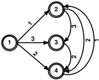
Example 4. Consider the C&LEX ( X , Y , C ) constraint where the C is REGULAR ( A , X ) and A is the automaton presented in Figure 1. Domains of variables are X [1] ∈ { 1 , 2 } , X [2] ∈ { 1 , 3 } , X [3] ∈ { 2 } and Y [1] ∈ { 1 , 2 , 3 } , Y [2] ∈ { 1 , 2 } , Y [3] ∈ { 1 , 3 } .

Consider Algorithm 1 that finds the lexicographically smallest solution of the REGULAR constraint. At line 7 it invokes a DC propagator for the REGULAR constraint to ensure that an extension of a partial solution on each step leads to a solution of the constraint. To do so, it prunes all values that are inconsistent with the current partial assignment. We will show that for the REGULAR constraint values consistent with the current partial assignment can be found in O ( log ( d )) time.

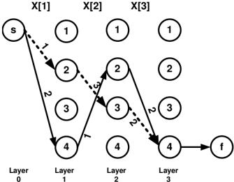
Let G x be a layered graph for the REGULAR constraint and L i = [ L [1] , . . . , L [ i ]] be a partial assignment at the i th iteration of the loop (lines 4 - 6, Algorithm 6). Then L i corresponds to a path from the initial node at 0 th layer to a node q i j at i th layer. Clearly, values of X [ i +1] consistent with the partial assignment L i are labels of outgoing arcs from the node q i j . We can find the label with the minimal value in O ( log ( d )) time. Algorithm 6 shows pseudo-code for REGULAR min ( A , L , X ) . Figure 2 shows a run of REGULAR min ( A , L , X ) for variables X in Example 4. The lexicographically smallest solution corresponds to dashed arcs.

Algorithm 6 REGULAR min ( A , L , X ) 1: procedure REGULAR min ( A : in, L : out, X : in ) 2: Build graph G x ; 3: q [0] = q 0 0 ; 4: for i = 1 to n do 5: L [ i ] = min { v j | v j ∈ outgoing arcs ( q [ i -1]) } ; 6: q [ i ] = t A ( q [ i -1] , L [ i ]) ; /triangleright t A is the transition function of A . 7: return L ;

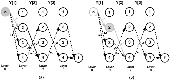
The time complexity of Algorithm 2 for the REGULAR constraint is also O ( nT ) . The algorithm works with the layered graph rather than original variables. On each step it marks edges that occur in feasible paths in G x that are lexicographically greater than or equal to L . Figure 3 shows execution of C&LEX lb ( X l , Y , REGULAR ) for vari-

ables Y and the lexicographically smallest solution for X , X l = (1 , 3 , 2) , from Example 4. It starts at initial node s and marks all arcs on feasible paths starting with values greater than X l [1] = 1 (that is 2 or 3 ). Figure 3(a) shows the removed arc in gray and marked arcs in dashed style. Then, from the initial node at 0 th layer it moves to the 2 nd node at the 1 st layer (Figure 3 (b)). The algorithm marks all arcs on paths starting with a prefix greater than [ X l [1] , X l [2]] = [1 , 3] . There are no such feasible paths. So the MarkConsistentArcs algorithm does not mark extra arcs. Finally, it finds that there is no outgoing arc from the 2 nd node at 2 nd layer labeled with 3 and stops its marking phase. There are two unmarked arcs that are solid gray arcs at Figure 3 (b). The algorithm prunes value 1 from the domain of Y [1] , because there are no marked arcs labeled with value 1 for Y [1] . Algorithm 8 shows the pseudo-code for C&LEX lb ( L , X , REGULAR ) . Note that the MarkConsistentArcs algorithm for the REGULAR constraint is incremental. The algorithm performs a constant number of operations (deletion, marking) on each edge. Therefore, the total time complexity is O ( nT ) at each invocation of the C&LEX lb ( L , X , REGULAR ) constraint.

Algorithm 7 Mark consistent arcs

1: procedure MarkConsistentArcs ( G x : out, q : in ) 2: Mark all arcs that occur on a path from q to the final node;

Algorithm 8 C&LEX lb ( L , X , REGULAR )

/negationslash

1: procedure C&LEX lb ( L : in, X : out, REGULAR : in ) 2: Build graph G x ; 3: q [0] = q 0 0 ; 4: q L = 0 ; 5: for i = 1 to n do 6: Remove outgoing arcs from the node q [ i -1] labeled with { min ( X [ i ]) , . . . , L [ i ] } ; 7: MarkConsistentArcs ( G x , q [ i -1]) ; 8: if ( ∃ a outgoing arc from q [ i -1] ) ∧ ( i = 1) then 9: mark arcs ( q [ k -1] , q [ k ]) , k = q L , . . . , i -1 ; 10: q L = i -1 ; 11: if L [ i ] / ∈ D ( X [ i ]) then 12: break; 13: q [ i ] = T A ( q [ i -1] , L [ i ]) ; /triangleright T A is the transition function of A . 14: if ( i == n ) then 15: mark arcs ( q [ k -1] , q [ k ]) , k = q L , . . . , n ; 16: for i = 1 to n do 17: Prune ( { v j ∈ D ( X [ i ]) | unmarked ( v j ) } ) ;

The second algorithm that we propose represents the C&LEX ( X , Y , REGULAR ) as a single automaton that is the product of automata for two REGULAR constraints and an automaton for LEX. First, we create individual automata for each of three constraints. Let Q be the number of states for each REGULAR constraint and d be the number of states for the LEX constraint. Second, we interleave the variables X and Y , to get the sequence X [1] , Y [1] , X [2] , Y [2] , . . . , X [ n ] , Y [ n ] . The resulting automaton is a product of individual automata that works on the constructed sequence of interleaved variables.

The number of states of the final automaton is Q ′ = O ( dQ 2 ) . The total time complexity to enforce DC on the C&LEX ( X , Y , REGULAR ) constraint is thus O ( nT ′ ) , where T ′ is the number of transitions of the product automaton. It should be noted that this algorithm is very easy to implement. Once the product automaton is constructed, we encode the REGULAR constraint for it as a set of ternary transition constraints [10].

The third way to propagate the C&LEX ( X , Y , REGULAR ) constraint is to encode it as a cost REGULAR constraint. W.L.O.G., we assume that there exist only one initial and one final state. Let G x be the layered graph for REGULAR ( X ) and G y be the layered graph for REGULAR ( Y ) . We replace the final state at n +1 th layer in G x with the initial state at 0 th layer at G y . Finally, we need to encode LEX ( X , Y ) using the layered graph. We recall that the LEX ( X , Y ) constraint can be encoded as an arithmetic constraint ( d n -1 X [1] + . . . + d 0 X [ n ] ≤ d n -1 Y [1] + . . . + d 0 Y [ n ]) or ( d n -1 X [1] + . . . + d 0 X [ n ] -d n -1 Y [1] -. . . -d 0 Y [ n ] ≤ 0) , where d = | ⋃ n i =1 D ( X [ i ]) | .

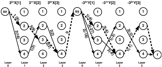
In turn this arithmetic constraint can be encoded in the layered graph by adding weights on corresponding arcs. The construction for Example 4 is presented in Figure 4. Values in brackets are weights to encode the LEX ( X , Y ) constraint. For instance, the arc ( s x, 2) has weight 9 . The arc corresponds to the first variable with the coefficient d 2 , d = 3 . It is labeled with value 1 . The weight equals 1 × d 2 = 9 . More generally, an arc between the k -1 th and k th layers labeled with v j is given weight v j d n -k . Note that the weights of arcs that correspond to variables Y are negative. Hence, the C&LEX ( X , Y , REGULAR ) constraint can be encoded as a cost REGULAR ([ A , A ] , [ X , Y ] , W ) constraint, where W is the cost variable, [ A , A ] are two consecutive automata. W has to be less than or equal to 0 . Consider for example the shortest path through the arc ( sy, 2) . The cost of the shortest path through this arc is 3 . Consequently, value 1 can be pruned form the domain of Y [1] .

The time complexity of enforcing DC on the cost REGULAR ([ A , A ] , [ XY ] , W ) is O ( nT ) , where d = | ⋃ n i =1 D ( X [ i ]) | and T is the number of transitions of A . 1 Again, the use of large integers adds a linear factor to the complexity, so we get O ( n 2 T ) .

1 Note that we have negative weights on arcs. However, we can add a constant d n to the weight of each arc and increase the upper bound of W by this constant.

4 Experimental results

To evaluate the performance of the proposed algorithms we carried out a series of experiments nurse scheduling problems (NSP) for C&LEX ( X , Y , SEQUENCE ) and C&LEX ( X , Y , REGULAR ) constraints. We used Ilog 6.2 for our experiments and ran them on an Intel(R) Xeon(R) E5405 2 . 0 Ghz with 4 Gb of RAM. All benchmarks are modeled using a matrix model of n × m variables, where m is the number of columns and n is the number of rows.

The C&LEX ( X , Y , SEQUENCE ) constraint. The instances for this problem are taken from www.projectmanagement.ugent.be/nsp.php. For each day in the scheduling period, a nurse is assigned to a day, evening, or night shift or takes a day off. The original benchmarks specify minimal required staff allocation for each shift and individual preferences for each nurse. We ignore these preferences and replace them with a set of constraints that model common workload restrictions for all nurses. Therefore we use only labor demand requirements from the original benchmarks. We also convert these problems to Boolean problems by ignoring different shifts and only distinguishing whether the nurse does or does not work on the given day. The labor demand for each day is the sum of labor demands for all shifts during this day. In addition to the labor demand we post a single SEQUENCE constraint for each row. We use a static variable ordering that assigns all columns in turn starting from the last one. Each column is assigned from the bottom to the top. This tests if propagation can overcome a poor branching heuristic which conflicts with symmetry breaking constraints. We used six models with different SEQUENCE constraints posed on rows of the matrix. Each model was run on 100 instances over a 28 -day scheduling period with 30 nurses. Results are presented in Table 1. We compare C&LEX ( X , Y , SEQUENCE ) with the decomposition into two SEQUENCE constraints and LEX. In the case of the decomposition we used two algorithms to propagate the SEQUENCE constraint. The first is the decomposition of the SEQUENCE constraint into individual AMONG constraints ( AD ), the second is the original HPRS filtering algorithm for SEQUENCE 2 . The decompositions are faster on easy

2 We would like to thank Willem-Jan van Hoeve for providing us with the implementation of the HPRS algorithm.

instances that have a small number of backtracks, while they can not solve harder instances within the time limit. Overall, the model with the C&LEX ( X , Y , SEQUENCE ) constraint performs about 4 times fewer backtracks and solves about 80 more instances compared to the decompositions.

Table 1. Simplified NSPs. Number of instances solved in 60 sec / average time to solve.

	AD , LEX	HPRS , LEX	C&LEX
1 SEQUENCE(3,4,5)	46 / 1.27	46 / 2.76	74 / 1.44
2 SEQUENCE(2,3,4)	66 / 0.63	66 / 1.29	83 / 2.66
3 SEQUENCE(1,2,3)	20 / 0.54	20 / 1.04	34 / 3.17
4 SEQUENCE(4,5,7)	78 / 1.36	77 / 2.31	82 / 2.43
5 SEQUENCE(3,4,7)	55 / 0.55	55 / 1.07	58 / 1.53
6 SEQUENCE(2,3,5)	19 / 5.38	18 / 8.27	31 / 1.74
solved/total	284 /600	282 /600	362 /600
avg time for solved	1.230	2.194	2.147
avg bt for solved	18732	16048	4382

Table 2. NSPs. Number of instances solved in 60 sec / average time to solve.

	REGULAR, LEX	C&LEX
12 hours break	30 / 9.31	93 / 2.59
12 hours break + 2 consecutive shifts	87 / 1.05	88 / 0.22
solved/total 117	/200	181 /200
avg time for solved	3.166	1.439
avg bt for solved	35434	1220

The C&LEX ( X , Y , REGULAR ) constraint. We implemented the second algorithm from Section 3.3, which propagates C&LEX ( X , Y , REGULAR ) using a product of automata for two REGULAR constraints and the automaton for the LEX constraint. C&LEX ( X , Y , REGULAR ) was compared with decomposition into individual REGULAR and LEX constraints. We used two models with different REGULAR constraints posed on rows of the matrix. Each model was run on 100 instances over a 7 -day scheduling period with 25 nurses. We use the same variable ordering as above. The REGULAR constraint in the first model expresses that each nurse should have at least 12 hours of break between 2 shifts. The REGULAR constraint in the second model expresses that each nurse should have at least 12 hours of break between 2 shifts and at least two consecutive days on any shift. Results are presented in Table 2. The model with the C&LEX ( X , Y , REGULAR ) constraint solves 64 more instances than decompositions and shows better run times and takes fewer backtracks.

5 Related and future work

Symmetry breaking constraints have on the whole been considered separately to problem constraints. The only exception to this of which we are aware is a combination of lexicographical ordering and sum constraints [11]. This demonstrated that on more difficult problems, or when the branching heuristic conflicted with the symmetry breaking, the extra pruning provided by the interaction of problem and symmetry breaking constraints is worthwhile. Our work supports these results. Experimental results show that using a combination of LEX and other global constraints achieves significant improvement in the number of backtracks and run time. Our future work is to construct a filtering algorithm for the conjunction of the Hamming distance constraint with other global constraints. This is useful for modeling scheduling problems where we would like to provide similar or different schedules for employees. We expect that performance improvement will be even greater than for the C&LEX constraint, because the Hamming distance constraint is much tighter than the LEX constraint.

References

1. Puget, J.F.: On the satisfiability of symmetrical constrained satisfaction problems. In: Proceedings of ISMIS'93. (1993) 350-361
2. Walsh, T.: Breaking value symmetry. In: Proc. of the 13th Int. Conf. on Principles and Practice of Constraint Programming, CP 2007. (2007) 880-888
3. Flener, P., Frisch, A.M., Kzlltan, B.H.Z., Miguel, I., Walsh, T.: Matrix modelling: Exploiting common patterns in constraint programming. In: Proc. of the Int. Workshop on Reformulating Constraint Satisfaction Problems. (2002) 27-41
4. Flener, P., Frisch, A., Hnich, B., Kiziltan, Z., Miguel, I., Pearson, J., Walsh., T.: Breaking row and column symmetries in matrix models. In: Proc. of 8th Int. Conf. on Principles and Practice of Constraint Programming. (2002) 462-476
5. Frisch, A., Hnich, B., Kiziltan, Z., Miguel, I., Walsh, T.: Global constraints for lexicographic orderings. In: Proc. of the 8th Int. Conf. on Principles and Practice of Constraint Programming (CP'02), van Hentenryck, P (2002) 93-108
6. Beldiceanu, N., Contejean, E.: Introducing global constraints in CHIP. Mathematical and Computer Modelling 12 (1994) 97-123
7. Pesant, G.: A regular language membership constraint for finite sequences of variables. In: Proc. of 10th Int. Conf. on Principles and Practice of Constraint Programming (CP'04). (2004) 482-495
8. Carlsson, M., Beldiceanu, N.: Arc-consistency for a chain of lexicographic ordering constraints. TR T-2002-18, Swedish Institute of Computer Science (2002)
9. Hoeve, W.J.v., Pesant, G., Rousseau, L.M., Sabharwal, A.: Revisiting the Sequence Constraint. In: Proc. of the 12th Int. Conf. on Principles and Practice of Constraint Programming (CP '06). (2006) 620-634
10. Quimper, C.G., Walsh, T.: Global Grammar constraints. In : Proc. of the 12th Int. Conf. on Principles and Practice of Constraint Programming. (2006) 751-755
11. Hnich, B., Kiziltan, Z., Walsh, T.: Combining symmetry breaking with other constraints: lexicographic ordering with sums. In: Proc. of the 8th Int. Sym. on the Artificial Intelligence and Mathematics. (2004)