Composition of Probability Measures on Finite Spaces

Radim Jirou!!ek"

Laboratory of Intelligent Systems University of Economics, Prague and Institute of Information Theory and Automation Academy of Sciences of the Czech Republic

Abstract

Decomposable models and Bayesian net­ works can be defined as sequences of oligo­ dimensional probability measures connected with opemtors of composition. The prelim­ inary results suggest that the probabilistic models allowing for effective computational procedures are represented by sequences pos­ sessing a special property; we shall call them perfect sequences.

The present paper lays down the elementary foundation necessary for further study of it­ erative application of operators of composi­ tion. We believe to develop a technique de­ scribing several graph models in a unifying way. We are convinced that practically all theoretical results and procedures connected with decomposable models and Bayesian net­ works can be translated into the terminology introduced in this paper. For example, com­ plexity of computational procedures in these models is closely dependent on possibility to change the ordering of oligo-dimensional mea­ sures defining the model. Therefore, in this paper, lot of attention is paid to possibility to change ordering of the operators of composi­ tion.

1 NOTATION

Let {Xi};EV be a finite system of finite sets. We shall deal with probability measures on the Cartesian prod­ uct space

and its subspaces

"E-mail: [email protected]

for L C V.

Consider K � L � V and a probability measure P defined on XK. By II(L) we shall denote the set of all probability measures defined on X£. Similarly, n<Ll(P) will denote the system of all extensions of the measure P to measures on XL:

where Q(K) denote the marginal measure of the mea­ sure Q on XK.

Now, let us introduce an operator 1> of composition. To make it clear from the very beginning, let us stress that it is just a generalization of the idea of comput­ ing the three-dimensional distribution from two two­ dimensional ones introducing the conditional indepen­ dence:

Consider two probability measures P E II(J) and Q E fi(K), such that Q(JnK) dominates1 p(JnK) ; in symbol:

p(JnK) , Q ( J n K) denote again the marginal measures of P, Q respectively, on XJnK. The ( right ) composition of these two measures is defined by the formula

1 The concept of dominance (or absolute continuity) P 4:: Q on finite space X s i m plifi e s to

Since we assume p(JnK) « Q(J n K), if f or any x E X( J n K) Q ( J n K)(x) = 0 then there is a product of two zeros in the nominator and we take, quite naturally,

If J n K = 0 then Q(JnK) = 1 and the formula degenerates to a simple product of P and Q.

It is obvious from this definition that P 1> Q is a proba­ bility measure from II(JuK) and that its marginal mea­ sure (PI> Q)(Jl equals P. In case p(JnK) %:. Q ( J n K) the expression P 1> Q remains undefined.

Example

Let us illustrate by a simple example difficulties which can occur when p(J n K ) %:. Q ( KnJ ) .

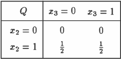
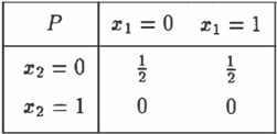
Consider the measures P E fi({1, 2 }) and Q E fi({ 2 · 3} ) given in the following tables.

Q	:1:3= 0	X3= 1
X2= 0	0	0
X2= 1	1 2	1 2

The reader can easily see that for any x E X{l , 2 ,3 } , X= ( x t ,:I:2,X3)

smce for X2 = 1 P(x2, X3) = 0 and for x2 = 0 Q(xt, x 2 ) = 0. <>

To avoid necessity of writing brackets distinguishing ex­ pression ((P 1> Q) 1> R) from (P 1> (Q 1> R)) we use also an analogous operator of left composition <1

which is properly defined whenever Q(JnK) « p ( J n K), otherwise it is again undefined. Hereafter we shall al­ ways assume that the operators are applied from left to right.

BASIC PROPERTIES 2

Lemma 1. Let K � L � V. For any probability measures P E n(K) and Q E II(L) such that P « Q(K),

and for any R E II( L l(P)

Proof.

The assertion directly follows from the definition of the operator 1> which can be for the current situation writ­ ten

From this formula it follows evidently that for any x E XL

which proves that P 1> Q « Q.

Analogously, let R E fi(Ll(P) be dominated by Q. Con­ sider an x E XL for which

where x(K) for x E XL denote the projection of x into the subspace X K . That means that either P(x(K)) = 0 or Q(x) = 0 ( or both). If P(x(K)) = 0 then R{Kl(x ( Kl) = 0 as R(K) equals p since R E nL(P). Therefore also R(x) = 0. On the other hand, if Q(x} = 0 then R(x) = 0 because R is dominated by Q. 0

In the proofs, we shall often compute a marginal mea­ sure from a measure defined as a composition of two ( or several ) oligo-dimensional measures. Therefore, it is important to realize that generally

As a simple example can serve

Nevertheless, the following simple assertion presents a sufficient condition under which the equality in the above expression holds.

Lemma 2. Let K, L, M C V. If M :J K n L than for any probability measures P E rr ( K) a ;;-d Q E [l ( L)

Proof.

To prove this, it is enough to marginalize ( P 1> Q ) as, for example, in the following way.

D

3 ITERATIONS OF THE OPERATORS OF COMPOSITION

We shall say that a pair of measures P1 E rr(K 1 ) , Pz E II (K o ) is consistent if

Directly from the definition of the operators <land 1> we get the following trivial assertion.

Lemma 3. Let for P1 E II (K t ) and P2 E II( K ,) either pfK1nK2) << p J K 1 n K 2) or pJK,nK,) « pf K ,n K,) P t and P2 are consistent if and only if

The situation becomes somewhat more complicated when the operators are applied (at least) twice. It is clear that generally 2

Now, let us present a few lemmata saying under which conditions some of these equalities hold. Whenever in this section we shall use probability measures P1, P2, P3, we shall assume that P; E n (K ; ) fori= 1, 2, 3.

Lemma 4. If Kt 2 ( !<2 n K3) then

2 As said above, operators t> and <1 are always applied from left to right.

P r oo f.

Under the assumption K1 2 (K2 n Ka)

and therefore the expressions

The next assertion expresses a very important property distinguishing left and right operators of composition. Namely, the operator of right composition 1> can be sub­ stituted by an operator @K, depending on a set K, si­ multaneously with changing the ordering of operations. Let us mention that no analogous operator exists for the operator of left composition <J.

Theorem 1. If P,, Pz and P3 are such that P11> P21> P3 is defined then

where

IS a probability measure on XK,uK,u ( K1nK3) XK ,u K 2· In the following computations of its marginal measure on XK,n(K,u K ,) we have to sum over x(K,uK,)\K,· Therefore, y ( K) for y E XK,uK, will de­ note its projection into XK. Analogous meaning are those of the symbols x (K ) and z(K).

For each y E Xk2uK3

And thus

which finishes the proof.

Corollary 1. If K2 2 (K ∩ Kg) then

and thus also

Proof.

The assertion is an immediate consequence of the fact

Lemma 5. If P1 and P2 are consistent then

Proof.

Since we assume K2 2 (K n K3)

and therefore

b d. h . p (K1nK2) ecause, accor mg to t e assumptiOns, 1 p J K,nK,) and J(3 n (Kr u K2) = /{3 n /{2 · 0

Lemma 6. If P1 and P3 are consistent then

0

Proof. Since

and

these two e xpr e ssion s are e q u iva l ent because under the given assumptions

The following Lemma is the o n ly assertion presented in this paper expressing a condition allowing to change the ordering of operations of composition that does not require a spec i al form of sets I<;. It is based only on a s p e cial form of conditional independence of measures P2 an d P3 and coincidence of respective conditional mea­ sures.

Lemma 7. If

then

Proof.

and

The denominators in both expressions equal each to other as

Therefore if one of the expressions Pt1>P21>Pa, Pti>Pat>P2 is defined then the other one must be defined, too, and then

Corollary 2. If P2 and Pa are consistent and for both i = 2,3

Proof

We shall only verify that all the assumptions of the preceding Lemma are fulfilled.

follows immediately from the consistency of P2, P3.

Moreover, under t h e giv e n assumptions

and therefore

for b ot h i = 2, 3.

4 GRAPH MODELS

This section should give a hint to answering the ques­ tion why we w e r e so much interested in finding con­ ditions under which changing an ordering of the op­ erations of composition does not influence the result­ ing measure. We shall assume that P; E IT (K ; ) for i = 1, . . . , n, and, moreover, that

The reader familiar with Bayesian networks and decom­ posable m o dels can immediately see that both these probabilistic models can be expressed in our notation as

An application of such a probabilistic model Q = P1 t> P2 t> · · · t> Pn to inference, i.e. for computation of a ( say ) conditional probability Q(Xr = aiX� = b) is simple if, for example, s E I< 1, r E Km and no I<m+l, Km+2, ... , I<n contains any of the indices r and s. On the contrary, however, the computational pro­ cedure can become extremely complex if s E Kn and r E Km for some m # n. Therefore, sequencies in which the ordering of the oligo-dimensional measures can be changed without changing the resulting multi­ dimensional measure are of great importance. Of great importance are also the perfect sequences introduced below.

We shall say that an ordered sequence of probability measures P1, ... , Pn is perf ect if

For these sequences the following two simple assertions hold. The first one is an immediate consequence of an inductive application of Lemma 3.

Lemma 8. Let Pt t> P2 t> ... t> Pn be defined. The sequence P1, P2, . . . , Pn is perfect if and only if the pair of measures ( P1 t> · · · t> P m-l) and P m are consistent for allm=2,3, . . . ,n. 0

Theorem 2. Let P1, P2, ... , Pn be a perfect sequence of oligo-dimensional probability measures. Then

Consider any m E 1, . .. , n- 1} and denote Q :::: Pt f>

Proof. { ... t> Pm. All distributions

have Q for their marginal measure and thus P1 t> ... t> Pn = Qt>Pm+t t> ... ,t>Pn E IT(Vl(Q) which proves the assertion 2.

Since, according to the perfectness of P1, . . . , Pm,

it is clear that

where K:::: Kt U .. . UKm. From Ptt> ... t>Pn E n(Vl( Q) and Q E fi( K )(Pm), we get immediately P1 t> ... t> P,. E rr ( V ) (Pm)· Since m ::::; n1 was arbitrary and Pt t> ... t> Pn E rr ( Vl(Pn) follows from the perfectness condition, we have finished the first part of the proof, too. 0

Thus, like for Bayesian networks and decomposable models, marginalization for perfect sequences can be done by a simple neglect of a "tail" of the sequence. Moreover, the direct consequence of the preceding as­ sertion is the fact that each Bayesian network

can be transformed into a perfect sequence.

Corollary 3. If Ptt> ... f>Pn is defined then the sequence Q1, ... , Qn computed by the following process

is perfect and

From a classical result of Kellerer ( Kellerer 1964 ) it follows almost directly that for a sequence of pairwise consistent measures P1, ... 1 Pn such that the sequence K 1, K 2, .. . 1 I< n meets the running intersection prop­ erty:

the sequence Pt1 · · · , Pn, defining a decomposable model

is perfect, too.

In the abstract, we expressed our conviction that most of theoretical results and procedures connected with Bayesian networks and decomposable models can be translated into the terminology of perfect sequences. To support this statement, let us conclude the paper by describing the procedure introduced by Lauritzen and Spiegelhalter (Lauritzen, Spiegelhalter 1988) and known under the name of local computations. This pro­ cedure is, in fact, nothing else than a transformation of a Bayesian network into a decomposable model.

Procedure

Let Pt, P2, . . · , Pn be a perfect sequence of oligo­ dimensional measures and (Lt, L2, ... , Lm) be an arbitrary decomposable covering ofV (i.e. L1, ... , Lm meets the running intersection property and ( £1 U ... U Lm) = V) such that

The index j, existence of which is guaranteed by the above condition, will be denoted by b( i) in the sequel (if there are more than one such j, b(i) is an arbitrary of them). Compute m x n oligo-dimensional measures R(l,l)· ... , R (l, m )1 R(2,1)· ... , R (n,m)· For i = 1 com­ pute

For i > 1 compute

To compute R(i,j) f o r i > 1 and j ::j:. b(i) find an ordering

such that Lit, . . . , Lim meets the running intersection property (such an ordering always exists). Then for each k > 1 there exists e < k for which

and then R(i.jk) can be computed

Theorem 3. Let a perfect sequence P1, P2, . .. , Pn, a decomposable covering L 1, .. . , Lm of V, and measures R(i,j) ( i = 1, ... , n, j = 1, ... , m ) be as in Procedure.

Then the measures R(i,j) are consistent with the mea­ sure P11> . . . I> P; for all i = 1, . . . ,n, j = 1, . . . ,m.

Proof.

When proving the assertion we shall proceed in the three steps: (a) for i = 1, (b) for i > 1 and j = b(i), and (c) for remaining indices i,j.

(a) The fact that all R(l,j) are consistent with P1 fol­ lows directly from

(b) Now, assume that the assertion holds for a fixed i, ( 1 ::; i < n). Thus, R(i,b( i+t)) must be consistent with P1 1> ... 1> P;, which means, in this case,

Since Lb(i+t) 2 K;+l 2 K;+t n (Kt U . .. UK;) we get from Lemma 2

(c) To conclude the proof consider two indices i, (1 ::5 i < n ) and k, (1 < k ::; m ) and assume that the assertion holds for all R(i,j )· j = 1, . .. , m and also for R(i+l,j.), R(i+l,il)· ... , R (i + l , ik-d · where it = b( i), . . . , im is the ordering from Procedure. We shall prove that it holds also for R(i+l,j·)·

In accordance with Procedure, denote e that index for which

Let us compute

for any K such that K n Li· � K;+1 n L; ·.

As

we can take I< = Lj· n Ljc in the last equality. Since we assume that R(i+t.it) is consistent with P1 1> · · · 1> P;+l we can thus substitute (P1 t> · · · 1> Pi+t)(Li·nK) by R (Li·nLicl h " h fi · h th f ( i+ l ,ic) , w 1c ms es e proo . o

Theorem 4. Let a perfect sequence P1, P2, ... , Pn, a decomposable covering L1, . .. , Lm of V, and measures

R(i,j) (i = l, . . . ,n, j = 1, . . . , m ) be as in Procedure. Then R(n,I)· ... , R ( n,m) is a perfect sequence, too, and

Proof

This assertion follows directly from the preceding The­ orem and the fact (cf. e.g. Theorem 1.5.7 in (Hajek et al. 1992)) that if two measures can be expressed as products of functions defined on XL1, · · · , XLm and their marginals on these subspaces coincide then these measures are equivalent. 0

5 CONCLUSIONS

We have presented a new apparatus based on the op­ erators of left and right compositions. Though the op­ erators are defined by almost identical formulae they substantially differ when used iteratively to compose sequences of probabilistic measures. The difference con­ sists mainly in computational complexity of t h e respec­ tive processes. In contrast to the operator of right com­ position t>, iterative application of the operator of left composition <J rather often leads to computationally in­ tractable procedures because of increasing dimension­ ality of the measures from which the normalization fac­ tors are computed. Another noteworthy difference is an existence of the operator @K guaranteed by The­ orem 1. Let us mention that the existence of this op­ erator is, in a sense, closely connected with ideas of Bayesian network marginalization (by nodes deletion and edges reversal) proposed by R. Shachter (Shachter 1986a, 1986b, 1988).

The probabilistic models described by perfect sequences of {oligo-dimensional) probability measures embody Bayesian networks (and, naturally, decomposable mod­ els, too). We conjecture, that these models constitute the very class of models for which effective computa­ tional procedures can be found. Therefore, in the fu­ ture, we shall concentrate to algoritmization of these processes for which the theoretical background is given by assertions in section 3.

Acknowledgments

This work was supported by the grant of Ministry of Education of CR no. VS96008.

References

Csiszar, I. (1975). !-divergence geometry of proba­ bility distributions and minimization problems. Ann. Probab., 3, pp. 146-158.

Hajek, P., Havranek, T. and Jirousek R. ( 1 99 2 ) . Un­ certain Information Processing in Expert Systems. CRC Press, Inc., Boca Raton.

Jensen, F. V. ( 1996). Introduction to Bayesian Network. UCL Press, London.

Kellerer, H.G. (1964). Verteilungsfunktionen mit gegeben Marginalverteilungen. Z. Warhsch. Verw. Ge­ biete, 3, pp. 2472 70.

Lauritzen, S.L., Spiegelhalter, D. (1988). Local compu­ tations with probabilities on g r a phi c al structures and their applications to expert systems. J. Roy. Stat. Soc. Ser. B., 50, pp 157-189.

Pearl, J. (1988). Probabilistic Reasoning in Intelligence Systems: Networ k s of Plausible Inference. Morgan­ Kaufmann, San Mateo, CA.

Shachter, R.D. (1986a). Evaluating influence diagrams. Oper. Res., 3 4 , pp 871-882.

Shachter, R.D. ( 1986b). Intelligent probabilistic infer­ ence. In: Uncertainty in Artificial Intelligence (L.N. Kana!, J.F. Lemmer (eds.)). North Holland, Amster­ dam, pp 371-382.

Shachter, R.D. (1988). Probabilistic inference and in­ fluence diagrams. Oper. Res., 3 6 , pp 589-604.