Computational Advantages of Relevance Reasoning in Bayesian Belief Networks

Yan Lin

University of Pittsburgh Intelligent Systems Program Pittsburgh, PA 1.5260 [email protected]. edu

Abstract

This paper introduces a computational framework for reasoning in Bayesian belief networks that derives significant advantages from focused inference and relevance reason­ ing. This framework is based on d-separation and other simple and computationally effi­ cient techniques for pruning irrelevant parts of a network. Our main contribution is a technique that we call relevance-based decom­ position. Relevance-based decomposition ap­ proaches belief updating in large networks by focusing on their parts and decompos­ ing them into partially overlapping subnet­ works. This makes reasoning in some in­ tractable networks possible and, in addition, often results in significant speedup, as the to­ tal time taken to update all subnetworks is in practice often considerably less than the time taken to update the network as a whole. We report results of empirical tests that demon­ strate practical significance of our approach.

1 Introduction

Emergence of probabilistic graphs, such as Bayesian belief networks (BBNs) [Pearl, 1988] and closely re­ lated influence diagrams [Shachter, 1986] has made it possible to base uncertain inference in knowledge­ based systems on the sound foundations of probabil­ ity theory and decision theory. Probabilistic graphs offer an attractive knowledge representation tool for reasoning in knowledge-based systems in the presence of uncertainty, cost, preferences, and decisions. They have been successfully applied in such domains as di­ agnosis, planning, learning, vision, and natural lan­ guage processing.1 As many practical systems tend to be large, the main problem faced by the decision­ theoretic approach is the complexity of probabilistic

1 Some examples of real-world applications are described in a special issue of Communications of the A CM, on prac­ tical applications of decision-theoretic methods in AI, V o l . 38, No. 3, March 1995.

Marek J. Druzdzel

University of Pittsburgh Department of Information Science and Intelligent Systems Program Pittsburgh, PA 15260 marek@sis. pitt. edu reasoning, shown to be NP-hard both for exact infer­ ence [Cooper, 1990] and for approximate [Dagurn and Luby, 1993] inference. .

The critical factor in exact inference schemes is the topology of the underlying graph and, more specifi­ cally, its connectivity. The complexity of approximate schemes may, in addition, depend on factors like the a-priori likelihood of the observed evidenee or asymme­ tries in probability distributions. There are a number of ingeniously efficient algorithms that allow for fast belief updating in moderately sized models.2 Still, eaeh of them is subject to the growth in complexity that is generally exponential in the size of the model. Given the promise of the decision-theoretic approach and an increasing number of its practical applications, it is important to develop schemes that will reduce the computational complexity of inference. Even though the worst case will remain NP-hard, many practical eases may become tractable by, for example, exploring the properties of practical models, approximating the inference, focusing on smaller elements of the models, reducing the connectivity of the underlying graph, or by improvements in the inference algorithms that re­ duce the constant factor in the otherwise exponential complexity.

In this paper, we introduce a computational frame­ work for reasoning in Bayesian belief networks that derives significant advantages from focused inference and relevance reasoning. We introduce a technique called relevance-based decomposition, that computes the marginal distributions over variables of interest by decomposing a network into partially overlapping sub-networks and performing the computation in the identified sub-networks. As this procedure is able, for most reasonably sparse topologies, to identify sub­ networks that are significantly smaller than the en­ tire model, it also can be used to make computa­ tion in large networks doable, under practical limi­ tations of the available hardware. In addition, we demonstrate empirically that it can lead to signifi­ cant speedups in large practical models for the dus-

2 For an overview of various exact and approximate ap­ proaches to algorithms in BBNs see [Henrion, 1990].

tering algorithm [Lauritzen and Spiegelhalter, 1988, Jensen et al., 1990].

All random variables used in this paper are multiple� valued, discrete variables. Lower case letters (e.g., x) will represent random variables, and indexed lower� case letters (e.g., x;) .will denote their outcomes. In case of binary random variables, the two outcomes will be denoted by upper case (e.g., the two outcomes of a variable c will be denoted by C and C).

The remainder of this paper is structured as follows. Section 2 reviews briefly the methods of relevance rea� soning applied in our framework. Section 3 discusses in somewhat more depth an important element of rel� evance reasoning, nuisance node removal. Nuisance node removal is the prime tool for significant reduc­ tions of clique sizes when clustering algorithms are subsequently applied. Section 4 discusses relevance­ based decomposition. Section 5 presents empirical re­ sults. Finally, Section 6 discusses the impact of our results on the work on belief updating algorithms for Bayesian belief networks.

2 Relevance Reasoning in Bayesian Belief Networks

The concept of relevance is relative to the model, to the focus of reasoning, and to the context in which reasoning takes place [Druzdzd and Suermondt, 1994]. The focus is normally a set of variables of interest T (T stands for the target variables) and the wntext is provided by observing the values of some subset E {E stands for the evidence variables) of other variables in the model.

The cornerstone of most relevance-based methods is probabilistic independence, captured in graphical models by a condition known as d-separation lPearl, 1988], which ties the concept of conditional indepen­ dence to the structure of the graph. Informally, an evi­ dence node blocks the propagation of information from its ancestors to its descendants, but it also makes all its ancestors interdependent. In this sec.tion, we will give the flavor of simple algorithms for relevance-based reasoning in graphical models that we applied in our framework.

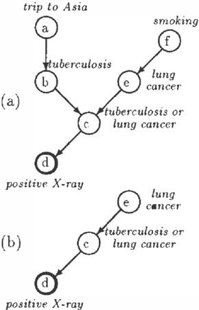
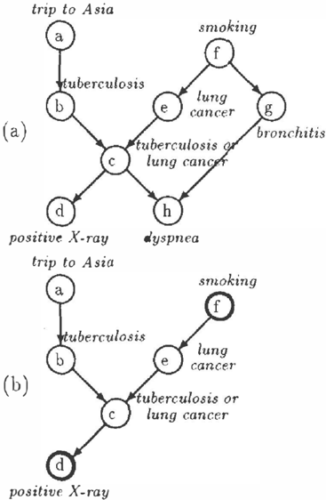
Parts of the model that are probabilistically indepen­ dent from the target nodes T given the observed ev­ idence E are computationally irrelevant to reasoning about T. Geiger et al. [1990b] show an efficient algorithm for identifying nodes that are probabilis­ tically independent from a set of target nodes given a set of evidence nodes. Removing such nodes can lead to significant savings in computation. Figure 1-a presents a sample network reproduced from Lauritzen and Spiegelhalter [I 988]. For example, node a is in­ dependent of node f if neither c, d, or h are observed (Figure 1-a). 1f nodes f and dare observed, node g will become independent of nodes a, b, c, and e, but nodes b and e will become dependent.

Figure 1: An example of relevance reasoning: removal of nodes based on the d-separation condition and bar­ ren nodes. Iff :::: { d,!} is the set of evidence nodes and T = {b, e} is the set of target nodes, then nodes h and g are barren.

The next step in reducing the graph is removal of barren nodes [Shachter, 1986]. Nodes are barren if they are neither evidence nodes nor target nodes and they have no descendants or if all their descendants are barren. Barren nodes may depend on the evi­ dence, but they do not contribute to the change in probability of the target nodes and are, therefore, wmputationally irrelevant. A simple extension to the algorithm for identifying independence can re­ move all barren nodes efficiently [Geiger et a/., 1 990b, Baker and Boult, 199 1]. Figure 1 illustrates the con­ struction of a relevant sub-network from the original network that is based on the d-separation c.riterion. Starting with the network in Figure 1-a, a set of ev­ idence nodes E = {d, !}, and a set of target nodes T == { b, e}, we obtain the network in Figure 1-b by re­ moving barren nodes g and h. {Once node h removed, we can also view node g as d-separated from T by the evidence£.) Networks (a) a n d (b) are equivalent with respect to computing the posterior probabilities ofT given£.

Schemes based on d-separation can be further en­ hanced by exploration of independences encoded im­ plicitly in conditional probability distributions, includ­ ing context-speeifir. independenr.es. Some examples of

such independences are listed by Druzdzel and Suer­ mondt [1994]. Other relevant work is by Boutilier et al. [1996], Heckerman [1990), Heckerman and Breese [1994], Smith et al. [199:3], and Poole [ 1 99:3].

The above example illustrates that relevance reasoning can yield sub-networks that are much smaller and less densely connected than the original network. The net­ work in Figure 1-b, in particular, is singly connected and can be solved in polynomial time. This can lead to dramatic improvements in performance, as most rele­ vance algorithms operate on the structural properties of graphs and their complexity is polynomial in the number of arcs in the network (see Druzdzel and Suer­ mondt [1994] for a brief review of relevance-based al­ gorithms).

There are two additional simple methods that we im­ plemented in our framework. The first method, termed evidence propagation, consists of instantiating nodes in the network if their values are indirectly implied by the evidence. The observed evidence may be causally sufficient to imply the values of other, as yet unob­ served nodes (e.g., if a patient is male, it implies that he is not pregnant). Similarly, observed evidence may imply other nodes that are causally necessary for that evidence to occur (e.g., observing that a car starts im­ plies that the battery is not empty). Each instanti­ ation reduces the number of uncertain variables and, hence, reduces the computational complexity of infer­ ence. Further, instantiations can lead to additional reductions, as they may screen off other variables by making them independent of the variables of interest.

The second method involves absorbing instantiated nodes into the probability distributions of their chil­ dren. Once we know the state of an observed node, the probabilities of all other states becomes zero and there is no need to store distributions which depend upon those states in its successors. We can modify the probability distribution of its successors and remove the arcs between them. The practical significance of this operation is that the conditional probability ta­ bles bec.ome smaller and this reduces both the memory and computational requirements. Evidence absorption is closely related to the operation by that name in the Lauritzen and Spiegelhalter's [ 1 988] clustering al­ � orithm and has been stud.ied in detail by Shachter l1990].

We should remark here that in cases where all nodes belong to the target set T, most of the techniques re­ viewed in this section cannot reduce the size of any cliques in the network - since everything is relevant, nothing can be removed. Evidence absorption, how­ ever, removes all outgoing arcs of the evidence nodes and, thereby, reduces the size of some cliques and guar­ antees to produce less complex networks, unless all ev­ idence nodes are leaf nodes. Of course, the clustering algorithms can be improved to reduce the clique size in practice, but this reduction usually amounts to re­ duction in computation and not in memory size taken by a clique, as it is done after the network has been compiled into a clique tree. The evidence absorption scheme achieves such reduction before eonstruc.ting the junction tree. Lastly, we want to point out that evi­ dence absorption often results in more removal of nui­ sance nodes, whieh is the subject of the next section.

3 Nuisance Nodes

Druzdzel and Suermondt [1994] introduced a class of nodes called nuisance nodes and emphasized that they are also reducible by relevance reasoning. Nuisance nodes consist of those predecessor nodes . that do not take active part in propagation of belief from the evi­ dence to the target.

Before discussing removal of nuisance nodes, we will define them formally- we believe that this might help to avoid misunderstanding. Of the definitions below, trail, head-to-head node, and active trail are based on Geiger e.t al. [ 1990a].

Definition 1 (trail in undirected graph) A trail in an undirected graph is an alternating sequence of nodes and arcs of the graph such that every arc join.s the nodes immediately preceding it and following it.

Definition 2 (trail) A trail in a directed acyclic graph is an alternating sequence of arcs and nodes of the graph that form a trail m the underlying undirected graph.

Definition 3 (head-to-head node) A node c is called a head-to-head node with respect to a trail t if there are two consecutive arcs a ---+ c and c fb on t.

Definition 4 (minimal trail) A trail connecting a and b in which no node appears more than once is called a minimal trail between a and b.

Definition 5 (active trail) A trail connecting nodes a and b is said to be active given a set of nodes£. if {1) every head-to-head node with respect to t either is in £. or has a descendant in £. and {2) every other node on t is outside £.

Definition 6 (evidential trail} A minimal active trail between an evidence node e and a node n, given a set of nodes £., is called an evidential trail from 1:' to n given£..

In case of reducing a network for the sake of explana­ tion of reasoning, the original application of nuisance nodes, the assumption was that only the evidential trails from £. to T are relevant for explaining the im­ pact of£. on T. N uisanc.e node is defined with respect to T, £., and all evidential trails between them.

Definition 7 (nuisance node) A nuisance node, given evidence £. and target T, is a node that z.s com­ putationally related toT given£ but is not part of any evidential trail from any node in £. to any node in T.

Nuisance nodes are computationally related because they are ancestors of some nodes on a d-connecting path (please, note that they cannot be d-separated or barren, as they have to be computationally related). We will introduce the concept of nuisance anchor de­ fined as follows:

Definition 8 (nuisance anchor) A nuisance an­ chor zs a node on an evidential trail that has at least on e immediate predece.s.sor that is a nuisance node.

We will aim to remove entire groups of connected nui­ sanc-e nodes, which will be captured by the following two definitions:

Definition 9 (nuisance graph) A nuisance graph is a subgraph consisting of an anchor and all its nui­ sance ancestors.

Definition 10 (nuisance tree) A nuisance tree is a nuisance graph that is a polytree.

Since no barren nodes exist in a network that contains only computationally related nodes, it is a straight­ forward process to demonstrate that nuisance graphs consist of only ancestors of nuisance anchors.

Finally, it is convenient for the sake of explanation to define the concept of bold nuisance nodes:

Definition 11 (bold nuisance node) A nuisance node is called bold if it h as no ancestors.

The definition of nuisance nodes provides a straight­ forward criterion for identifying them in a graphical model. Identification of nuisance graphs can be per­ formed by a variant of the Depth-First-Search algo­ rithm that has complexity O(e), where e is the number of arcs in the network. The algorithm in Figure 2 for identifying nuisance nodes in directed acyclic. graphs is a revised version of the non-separable component algorithm (Even, 1979]. Since all descendant nodes of target or evidence in the (pruned) computational relevant subnetwork can not be nuisance nodes, we mark them ACTIVE first. Then following an arc from an active node to its parent, we find a non-separable component, which is a nuisance graph if it does not contain any active nodes.

To marginalize a nuisance graph into its anchor we need to know the joint probability distribution of t ho se nodes in the graph that are the anchor's parents. In ease the graph is a tree, the parents are independent and the tree can be reduced by a recursive marginaliza­ tion of its bold nuisance nodes until the entire nuisance tree is reduced.

Suppose (Figure :3-a) that the evidence set is £ = { d} and the target set is T = { e}. Nodes a and b form a nuisance tree with anchor at c and node f forms a one­ node nuisance tree with anchor in c. Nuisance nodes a and fare bold, In order to reduce both trees into their anchors, we need to successively marginalize their bold

Given: A computationally relevant Bayesian N e t w o r k net: a set of target nodes T a set of e vide nc e nodes £. void Mark_Nuisance_Nodes(net) em pty stack s; for each node n in the network do n.k := 0 if ( n is a descendant of target or evidence) then n.mark :=ACTIVE else n.mark := CLEAN for each arc in the network do arc.mark := UNVISITED while (there is still an ACT/ V E nodes n that has UNVISITED incident arcs to its parents) do v := n; v.f :=nil; push v to stack s; i := 1; v.k := i; v.l := i; repeat while (v has. UNVISITED incident arc ) do follow arc to find the node u arc.mark := VISITED if u.k = 0 then if u.k < v.l then v.l = u.k; else u.f := v; v := u; push v to stack s; i := i + 1; v.k := i; l.v := i end if ( v.f.k = 1 or v . l >= v.f.k) then pop all nodes from stack s down to (including) v; these nodes with v.f forms a non-separable set. if (no ACTIVE nodes in this set) then mark all nodes in this set NUISANCE else mark all nodes in this set ACTIVE else if ( v.l < v.f.l) then v.f.l := v.l v := v.f; until ( v .f = nil or v has no UNVISITED incident a rc ) end

nodes into their descendants, f into e, a into b, and finally b into c. The last operation, in particular, is performed using the following formulas:

An operation that is analogous to nuisance node removal in networks consisting of Noisy-OR nodes [Pearl, 1988] , is also performed by the Netview pro­ gram described by Pradhan, et al. [Pradhan et al., 1994].

Marginalization of nuisance graphs that are not nui­ sance trees is less straightforward: to be able to remove a nuisance graph, we need to first construct a new

conditional probability table for the nuisance anchor. Temporarily forgetting about the evidence present in the network, we condition on the non-nuisance par­ ents of the nuisance anchor and treat the nuisance an­ chor as a target node. The rest of the network below the nuisance anchor is computationally irrelevant to the target. Any standard inference algorithm can be used to compute the conditional probability distribu­ tion of the nuisance anchor, which can then be used to merge the entire nuisance graph into the anchor. When all parents of the nuisance anchor themselves are nuisance nodes, we can remove the entire nuisance graph by computing the prior probability distribution of the nuisance anchor. While computing the prob­ ability distribution over a nuisance anchor is hard in general, this probability distribution can be precom­ puted in advance for some of the those subnetworks that are potential nuisance graphs. Please, note that the probability distribution over a potential noise an­ chors is not conditioned on any evidence, which makes such precomputation feasible.

Removal of a nuisance tree originating from a nuisance anchor reduces one dimension of the conditional prob­ ability table (and hence, clique) containing the nui­ sance anchor and its remaining parents. In the case of nuisance graphs that are not trees, while their re­ moval may lead to significant computational advan­ tages, the computation related to establishing their marginal probability may be in itself complex. To make the marginalization of nuisance graphs worth­ while, it is possible to cache conditional probability tables for those cases that are commonly encountered. These cache tables can be computed at the time the model is constructed and stored for the efficiency of later reasoning. Please note that tables only at those nodes that are potential anchors (identified by the algorithm of Figure 2) need to be precomputed and stored.

4 Relevance-Based Decomposition

It is quite obvious that relevance rea.soning can lead to signific.ant computational sav i n g s if the reasoning is focused, i.e., if the user is interested only in a sub­ set of nodes in the network. (We report almost three orders of magnitude improvement in a very large rned� ical diagnostic network in Section 5.) Relevance-based methods can be very useful even if no target nodes are specified, i.e., when all nodes in a network are of interest. When the original network is large, comput­ ing the posterior distribution over all nodes may be­ come intractable: for example, due to excessive mem­ ory requirements of the clustering algorithm. [n such cases, we can attempt to divide the network into sev­ eral partially overlapping subnetworks, where all sets combined cover the entire network, Focusing on eac:h of these small subnetworks in separation leads eventu­ ally to updating the beliefs of all nodes in the network.

The main problem is, of course, dividing the network. We accomplish that by choosing at each step i a small set of target variables T; and pruning those nodes in the network that are not computationally relevant to updating the probability of T; given [. Since not all nodes in the network are computationally relevant to T;, the size of relevant subnetworks can be much smaller than that of the original network. The order in which the target sets T; are selected is crucial for the performance of the algorithm. Obviously, with a wrong choice ofT;, the subsets may overlap too much and lead to performance deterioration. lJ seful heuris­ tics that will minimize the overlap among various sub­ networks remain still to be studied. We have observed, however, that even with a very crude choice of the tar­ get sets T;, not only can we handle many intractable networks, but also decrease the total computation time in tractable networks. ( W e report four-fold increase in speed in Section 5.) This, of course, is not guaran­ teed and depends on the topology of the network. In very densely connected networks, everything may be relevant to everything, no matter what target set we choose. Such networks, however, would be intractable for any exac.t inference algorithm.

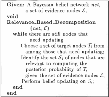
A sketch of the algorithm outlined informally above is given in Figure 4. We choose at each step i a set of tar­ get nodes T;. Subsequently, we use the relevance rea­ soning techniques outlined in Sections 2 and :3 to iden­ tify a s u bn e t w o r k that is relevant for computing the posterior probability ofT; g i v e n£ . Finally, we employ a standard inference algorithm to compute the pos­ terior probability distribution over the target nodes. Since in general the identified subnetwork will imlude other nodes than T; and £, we update a part of the network. We proceed by focusing on different network nodes from among those that have not yet been up-

dated until all nodes have been updated.

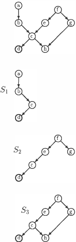
Figure 5 shows a simple example of relevance-based decomposition, given evidence node £ = { d} and the choice of targets in different steps: T1 = {a}, 72 = {g}, and 73 = {h}. We decompose the network into three subnetworks. Please note that network S'2 is a subset of .'h, which leads to redundant computation. We could avoid this by choosing h as a target before c.hoosing g.

5 Empirical Results

In this section, we present the results of an empm­ cal test of our relevance-based framework for Bayesian belief network inference. We focused our tests on the most surprising result: impact of relevance-based net­ work decomposition on the computational complexity of the inference. The algorithm that we used in all tests is an efficient implementation of the clustering algorithm that was made available to us by Alex Ko­ zlov. See Kozlov and Singh [1996] for details of the implementation and some benchmarks. We have en­ hanced Kozlov's implementation with relevance tech­ niques described in this paper. We have not included caching the probability distributions of nuisance an­ chors in our tests.

We tested our algorithms using the CPCS network, a multiply-connected multi-layer network consisting of 422 multi-valued nodes and covering a subset of the domain of internal medicine [Pradhan et a/., 1994). Among the 422 nodes, 14 nodes describe diseases, 3:3 nodes describe history and risk factors, and the re­ maining 375 nodes describe various findings related to the diseases. The CPCS network is among the largest real networks available to the research community at present time.

Our computer (a Sun Ultra-2 workstation with two 168Mhz UltraSPARC-1 CPU's, each CPU has a 0.5MB L2 cache, the total system RAM memory of

:384 MB) was unable to load, compile, and store the entire network in memory and we decided to use a sub­ set consisting of 360 nodes generated by Alex Kozlov for earlier benchmarks of his algorithm. This network is a subset of the full422 node CPCS network without predisposing factors (like gender, age, smoking, etc..). This reduction is realistic, as history nodes c.an usually be instantiated and absorbed into the network follow­ ing an interview with a patient.

We generated 50 test cases consisting of ten ran­ domly generated evidence nodes from among the find­ ing nodes defined in the network.3 For each of the test

3ln a dd i t i o n we c o n d u c t ed tests for different numbers of evidence n o d e s . Although the performance of our a!-

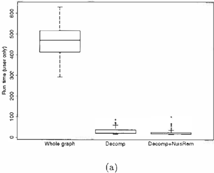
cases, we (1) ran the clustering algorithm on the whole network, (2) ran the relevance-based decomposition al­ gorithm without nuisance node removal, and (:)) ran the relevance-based decomposition algorithm with nui­ sance node removal. In case of the relevance-based de­ composition, we selected at eaeh step one target node from among those nodes that had not been updated. We always took the last node on the node list, which was ordered according to the partial order imposed by the graph structure (i.e., parents pr ec e d e d their chil­ dren on the list). This procedure gave preference to nodes dose to t he bottom of the graph. The results of our tests are presented in Figure 6 with the summary data in Table 1. It is apparent that the relevance­ based decomposition in combination with the c l u s ­ tering algorithm performed on average over 20 times faster than clustering algorithm applied to the entire network. This difference and the observed variance was s m a l l enough to reject possible differences due to chance at p < 10-38. Nuisance node removal ac­ counted on the average for over :30% improvement in speed ( p < 10-4).

Table 1: S u m m a r y simulation results for the CPCS network, n = .SO.

Jl	4'
(J"	15.927
Min	14.250
Median	17.825
Max	98.230

In addition to the CPCS network, we tested the relevance-based decomposition on several other large BBN models. One of these was a randomly generated highly connected network A [Kozlov and Singh, 1996] that we knew was rather difficult to handle for the clus­ tering algorithm. We have not performed tests for fo-

Table 2: Summary simulation results for the A net­ work [Kozlov and Singh, 1 996], n = 50.

		ecompos1twn
tt	• 1: .	.7
(J"	:37.074	48.430
Min	158.7.50	1.283
Median	20:�.87f)	7.208
Max	30.').817	331.483

cused inference for the A network, as the network was artificial and choosing target nodes randomly would be rather meaningless. Summary results of this test are presented in Table 2. The main reason why stan­ dard deviation is larger for the relevance-based decom- gorithrn deteriorated as more evidence nodes were added, the algorithm was still faster than belief updating on the entire network even for as many as 40 evidence nodes. We decided to report results for ten evidence nodes, which we believed to be typical for a diagnostic session with CPCS.

00S

400

000

200

Run time (user ony)

0

4

10

20

30

ir.dividual cases

(b)

Figure 6: Comparison of the c l u st e r in g algorithm ap­ pli e d to the whole network versus the clustering algo­ rithm enhanced with relevance-based decomposition and focused relevance, n = .50. Box-plot (a) and time series plot (b) topmost are the times for the whole network, middle for the relevance-based dewm­ position without nuisance node removal, and bottom, relevance-based decomposition with nuisance node re­ moval.

position algorithm was an outlier of :3:H .48:3 seeonds. The clustering algorithm took 264.7:3:3 seconds for this case. In no other of the 50 eases was the dustering al­ gorithm faster. We also run tests on several networks that we took from a student model of the Andes intelli­ gent tutoring system [Conati et a/., 1997] with similar results. Some of the Andes networks were too large to be solved by the clustering algorithm, but were up­ dated successfully by the relevanc.e-based decomposi­ tion. Performance differences in ease of random tests of tractable Andes networks were minimal and often relevance-based decomposition performed worse than the clustering algorithm applied to the whole network,

40

50

which confirms that the advantages of relevance-based decomposition are topology-dependent. Focused in­ ference based on relevance reasoning was, on the other hand, consistently orders of magnitude faster than be­ lief updating in the entire network.

One weakness of our experiments that we realized only recently is that we did not have full control over the triangulation algorithm used by the available imple­ mentation of the clustering a lg o rithm. We realized that the· triangulation algorithm did little in terms of optimizing the size of the junction tree and was sen­ sitive to the initial ordering of the nodes. Relevance algorithm run in the p reprocessing phase usually im­ pac te d this ordering. Still, we c.onsider it impossible that the observed differences in performance can be attributed to noise in triangulation algorithm - our results are too consistent for this to be a eompetitive rival hypothesis.

6 Discussion

Computational c om p l e x ity remains a major problem in application of probability t he o ry and decision the­ ory in k n owledge -ba se d systems. It is important to develop schemes that will reduce it even though the worst case will remain NP-hard, many practical cases may become tractable. In this paper, we pro­ posed a computational framework for belief updating in directed probabilistic graphs based on relevance rea­ soning that aims at reducing the size and connectiv­ ity of networks in cases where the i nf e r e nc e is focused on a subset of the network 's n o d es . We i ntroduced relevance-based decomposition, a scheme for comput­ ing the marginal distributions of target variables by decomposing the set of target variables into subsets, determining which of the model variables are relevant to those subsets given the new evidence, and perform­ ing the computation in the so-identified sub-networks.

As relevance-based decomposition can, for most reasonably sparse topologies, identify sub-networks that are significantly smaller than the entire model. Relevance-based decomposition can also be used to make c.omputation tractable in large networks. A somewhat surprising empirical finding is that this pro­ cedure often leads to s i g ni fi c a n t performance improve­ ment even in tractable networks, compared to exact inference in the entire network. One explanation of this finding is that relevance-based techniques are of­ ten capable of reducing the c.lique size at a small com­ putational cost. Roughly speaking, the clustering al­ )!;orithm constructs a junction tree, whose nodes de­ note partially overlapping dusters of variables in the original network. Each duster, or clique, encodes the marginal distribution over the set val( X) of the nodes ;t' in the cluster. The complexity of inference in the j unction tree is determined roughly by the size of the largest clique. Reducing the size of the junction tree and breaking large cliques can reduce the complexity of reasoning drastically. Another reason for the observed speedup is that smaller networks are more wrnpatible with the hardware r.ache on most computer configura­ tions and lead to faster computation by avoiding cache p a ge thrashing. For every corn pu ter system , there exist networks that do not fit in its cache or work­ ing memory. D e c o mpo si t i on described in t h i s paper w i l l often alleviate possible performance degradation in such cases.

Clustering algorithms aim at distributing the compu­ tational com])lexity between the process of cornpiling a graph, in which the pror.ess of triangularizing the graph is the most important, and belief updating. This is particularly advantageous when a domain model is static in the sense of no t b ei n g modified while entering evidence and processing probabilistic queries. Meth­ ods, as outlined i n this paper, seem to be not very suitable for such situations: the framework for rele­ vance r e a s o n in g presented in this paper always starts with the initial network and produces reduced net­ works that need to be c o mp i l e d from snatch. The cost for using this scheme and all relevance schemes that work on directed graphs is the c.ost to recompile relevant sub-networks into clique trees before compu­ tation. We have found that the relevance algorithms prove themselves worth the cost by sufficient savings in terms of reduced size and connectivity of the n e t ­ work. This can be further enhanced, as one of the reviewers suggested, by caching results of reasoning in overlapping subgraphs. Compilation of and reasoning with the reduced networks may achieve results faster than reasoning with the original network. Applica­ tion of the p r o p os e d schemes suggests that efforts be direc.ted at dev e l o ping efficient triangularization algo­ rithms that can approach optimality fast and can be used in real-time. Some hope for such schemes has been given in the recent work of Becker and Ueiger [ 1 996] .

We believe that the relevance-based preprocessing of networks will play a significant role in improving-the tractability of probabilistic inference in practical sys­ tems. T heir computational complexity is low and they can be used as an enhancement to any algorithm, even one that draws significant advantages from precompi­ lation of networks, such as the dustering algorithm used in all test runs in this paper.

Acknowledgments

This research was supported by the National Sci­ ence Foundation under Faculty Early Career Devel­ opment (CAREER) Program, grant I RI-9624629, a nd by ARPA's Computer Aided Education and T ra i n i n g Initiative under grant number N6600 1-9.5-C-8:367. We are grateful to Alex Kozlov for making his implemen­ tation of the clustering algorithm and several of his benchmark networks available to us. Malcolm Prad­ han and Max Henrion of the Institute for Decision Sys­ tems Research shared with us the CPCS network with a kind permission from the developers o f t h e I nt e r n i s t

system at the University of Pittsburgh. We are in­ debted to Jaap Suermondt and anonymous reviewers for insightful suggestions.

References

• [Baker and Boult, 1 991] Baker, Michelle and Boult, Terrance E. 199 1 . Pruning Bayesian networks for efficient computation. In Bonissone, P. P. ; Henrion, M.; Kana!, L.N.; and Lemmer, J .F., editors 1 99 1 , Uncertainty in Artificial Intelligence 6. Elsevier Sci­ ence Publishers B.V. (North Holland). 225�2:32.
• [Becker and Geiger, 1996] Becker, Ann and Geiger, Dan 1996. A sufficiently fast algorithm for find­ ing dose to optimal junction trees. l n Proceedings of the Twelfth A nnual Conference on Uncertainty in Artificial Intelligence (UAI�96), Portland, Oregon. 8 1�89.
• [Boutilier et a/. , 1 996] Boutilier, Craig; Friedman, Nir; Goldszmidt, Moises; and Koller, Daphne 1 996. Context-specific independence i n Bayesian networks. I n Proceedings of the Twelfth Annual Conference on Uncertainty in Artificial Intelligence (UAI�96}, Portland, Oregon. 1 15�1 2:3 .
• [ Conati ct a!. , 1 997] Conati , Cristina; Gertner, Abi­ gail; VanLehn, Kurt; and Druzdzel, Marek J . 1 997. On-line student m od el i ng for coached problem solv­ ing using Bayesian n e two r k s . In To Appear in Sixth International Conference on User Modeling, Sar­ dinia, Italy.
• [Cooper, 1990] Cooper, Gregory F. 1 990. The com­ putational complexity of probabilistic inference us­ ing Bayesian belief networks. Artificial Intelligence 42(2�:3) ::393�40.5 .
• [Dagum and Luby, 199:3] Dagum, Paul and Luby, Michael 199:3 . Approximating probabilistic infer­ ence in B ay es i a n belief networks is NP-hard. Ar­ t i ficial Int elligence 60 ( 1 ) : 1 4 1 - 1. 5:3.
• [Druzdzel and Suermondt, I 994) Druzdzel, Marek J . and Su e rm on d t , Henri J . 1 994. Relevance in proba­ bilistic models: "Backyards" in a "small world" . In Working notes of the A A A I-1994 Fall Symposium Series: Relevance, New Orleans, LA (An extended version of this paper is in preparation.). 60-63.
• [Even, 1979) Ev e n , Shimon 1 979. Graph algorithms. Computer Science Press, Potomac, MD.
• [Geiger et al. , 1 990a) Geiger, Dan; Verma, Thomas S.; and Pearl, Judea 1990a. d-Separation: From t heo ­ rems to algorithms. In Henrion, M . ; Shachter, R.D.; Kana!, L.N.; and Lemmer, J . F . , e ditor s l 9 90a, Un ­ cert ainty in A rtificial Intelligence. 5. Elsevier Science Publishers B.V. (North Holland) . 1 :39-148.
• [Geiger et al. , 1 990b] Geiger, Dan; Verma, Thomas S.; and Pearl , Judea 1990b. Identi­ fying independence in Bayesian networks. Networks 20(5):507-5:34.
• [Beckerman and Breese, 1994] Beckerman, David and Breese, John S. 1 994. A new look at causal indepen­ dence. In Proceedings of the Tenth A nnual Confer­ ence. on Uncertainty in Artificial Intelligence (UAI94}, Seattle, WA. 286-292.
• [Beckerman, 1 990) Beckerman, David 1990. Proba­ bilistic similarity networks. Networks 20(5):607-6:36.
• [Henrion, 1 990] Henrion, Max 1 990. An introduction to algorithms for inference in belief nets. In Hen­ rion, M . ; Shac.hter, R.D. ; Kana!, L.N.; and Lemmer, J . F . , editors 1 990, Uncertainty in Artificial Intel­ ligence 5. Elsevier Science Publishers B.V., North Holland. 129-1:38.
• [Jensen ei a/. , 1 990] J ensen, Finn Verner; Olesen, K r i s tian G . ; and Andersen , Stig Kjrer 1990. An alg eb ra of Bayesian belief universes for knowledge­ based systems. Networks 20(5):6:37-659.
• [Kozlov and Singh, 1 996) Kozlov , Alexander V. and Singh, Jaswinder Pal 1 996. Parallel implementa­ tions of pro b a b i l is t i c inference. IEEE Computer :3:340.
• [Lauritzen and Spiegelhalter, 1 988] Lauritzen, Stef­ fen L. and Spiegelhalter, David J . 1 988 . Local com­ putations with probabilities on graphical structures and their application to expert systems. Journal of the Royal Statistical Society, Series B (Methodolog­ ical) 50(2): 1 57�224.
• [Pearl, 1 988] Pearl, J udea 1 988 . Probabil!.stu : Rea.son­ ing in Intelligent Systems: Networks of Plausible Inference. Morgan Kaufmann Publishers, Inc., San Mateo, CA.
• [Poole, 1993) Poole, David 1 99:3 . Probabilistic Horn abduction and Bayesian networks. Artificial lntelli­ ge.nce 64( 1 ) :8 1- 129.
• [Pradhan et a/. , 1 994) Pradhan, Malcolm; Provan, Gregory; Middleton, Blackford; and Henrion , Max 1 994. Know ledge engineering for large belief net­ works. In Proceedings of the Tenth Annual Confer­ ence. on Uncertainty in Artificial Intelligence (U Al94}, Seattle, WA. 484-490. ·
• [Shachter, 1 986] Shachter, Ross D . 198'6. Evaluating influence diagrams. Operations Re.search :34(6):87 1882.
• [Shachter, 1 990) Shachter, Ross D. 1990. Evidence absorption and propagation through ev i d e n c e re­ versals. In Henrion, M . ; Shachter, R.D.; Ka n a! , L.N. ; and Lemmer, J . F . , editors 1 990, Uncertainty in Artificial Intelligence 5. Elsevier Science Publish­ ers B . V . , North Holland. 1 7:3-1 90 .
• [Smith e t al. , 1 99:3] Smith, J.E.; Holtzman, S.; and Matheson, J .E. 1 993. Structuring conditional re­ lationships in influence diagrams. Operation.s Re­ . s e arch 41(2):280-297.