Computational Investigation of Low-Discrepancy Sequences in Simulation Algorithms for Bayesian Networks

Jian Cheng & Marek J. Druzdzel

School of Information Sciences and Intelligent Systems Program

Decision Systems Laboratory University of Pittsburgh, Pittsburgh, PA 15260 {jcheng,marek}@sis.pitt.edu

Abstract

Monte Carlo sampling has become a major vehicle for approximate inference in Bayesian networks. In this paper, we investigate a fam­ ily of related simulation approaches, known collectively as quasi-Monte Carlo methods based on deterministic low-discrepancy se­ quences. We first outline several theoreti­ cal aspects of deterministic low-discrepancy sequences, show three examples of such se­ quences, and then discuss practical issues re­ lated to applying them to belief updating in Bayesian networks. We propose an algorithm for selecting direction numbers for Sobol se­ quence. Our experimental results show that low-discrepancy sequences (especially Sobol sequence) significantly improve the perfor­ mance of simulation algorithms in Bayesian networks compared to Monte Carlo sampling.

1 Introduction

Since exact inference in Bayesian networks is NP-hard [Cooper, 1990], approximate inference algorithms may for very large and complex networks be the only class of algorithms that will produce any result at all. A prominent subclass of approximate algorithms is the family of schemes based on Monte Carlo sampling (also called stochastic simulation or stochastic sam­ pling algorithms). The expected error of Monte Carlo sampling, fairly independent of the problem dimension (i.e., the number of variables involved), is of the order of N-1/2, where N is the number of samples. Ran­ dom point sets generated by Monte Carlo sampling show often clusters of points and tend to take wasteful samples because of gaps in the sample space. This observation led to proposing error reduction meth­ ods by means of determinate point sets, such as low­ discrepancy sequences. Low-discrepancy sequences try to utilize more uniformly distributed points. Appli­ cation of low-discrepancy sequences to generation of sample points for Monte Carlo sampling leads to what is known as quasi-Monte Carlo approaches. The er­ ror bounds in quasi-Monte Carlo approaches are of the order of (log N)d · N-1, where d is the problem dimension and N is again the number of samples gen­ erated. When the number of samples is large enough, quasi-Monte Carlo methods are theoretically superior to Monte Carlo sampling. Another advantage of quasi­ Monte Carlo methods is that their error bounds are deterministic.

Quasi-Monte Carlo methods have been successfully ap­ plied to computer graphics, computational physics, fi­ nancial engineering, and approximate integrals (e.g., [Niederreiter, 1992a, Morokoff and Caflisch, 1995, Paskov and Traub, 1995, Papageorgiou and Traub, 1997]). They have proven their advantage in low­ dimensionality problems. Even though some authors (e.g., [Bratley et al. , 1992, Morokoff and Caflisch, 1994]) believe that the quasi-Monte Carlo methods are not suitable for problems of high-dimensionality, tests by Paskov and Traub [1995] and Paskov [1997] have shown that quasi-Monte Carlo methods can be very effective for high-dimensional integral problems arising in computational finance. Papageorgiou and Traub [1997] have reported similarly good performance in high-dimensional integral problems arising in com­ putational physics, demonstrating that quasi-Monte Carlo methods can be superior to Monte Carlo sam­ pling even when the sample sizes are much smaller. These results rise the question whether quasi-Monte Carlo methods can improve sampling performance in Bayesian networks. To the best of our knowledge, ap­ plication of quasi-Monte Carlo methods to Bayesian networks has not been studied before. Of particu­ lar interest here are high-dimensionality problems, i.e., Bayesian networks with a large number of variables, as these are problems that cannot be solved using exact methods.

In this paper, we investigate the advantages of ap­ plying low-discrepancy sequences to existing sam­ pling algorithms in Bayesian networks. We first out­ line several theoretical aspects of deterministic quasi­ Monte Carlo sequences, show three examples of low­ discrepancy sequences, and then discuss practical is­ sues related to applying them to belief updating in Bayesian networks. We propose an algorithm for se­ lecting direction numbers for Sobol sequence. Our experimental results show that low-discrepancy se­ quences (especially Sobol sequence) can lead to sig­ nificant performance improvements of simulation al­ gorithms compared to existing Monte Carlo sampling algorithms.

In the following discussion, all random variables used are multiple-valued, discrete variables. Bold capital letters, such as X, A, denote sets of variables. Bold capital letter E denotes the set of evidence variables. Bold lower case letter e, is used to denote the observa­ tions, i.e., instantiations of the set of evidence variables E. Indexed capital letters, such as X;, denote random variables. Bold lower case letter a denotes a particu­ lar instantiation of a set A. Pa(X;) denotes the set of parents of node X;. \ denotes set difference. The no­ tation for low-discrepancy sequences will be clarified as introduced in the paper.

The remainder of this paper is organized as follows. Section 2 provides a brief introduction to the concept of discrepancy and to low-discrepancy sequences. Sec­ tion 3 presents construction methods for three pop­ ular low-discrepancy sequences - Halton, Sobol and Faure sequences. Section 4 discusses how these low­ discrepancy sequences can be used in Bayesian net­ works. We also propose an algorithm for selection of direction numbers for Sobol sequence. Section 5 re­ ports our empirical evaluation of quasi-Monte Carlo methods in Bayesian networks. Finally, Section 6 dis­ cusses the implications of our findings.

2 Discrepancy and Low-discrepancy Sequences

This section provides a brief introduction to the con­ cepts of discrepancy and low-discrepancy sequences as applied in quasi-Monte Carlo methods. Our exposition is based on that of Niederreiter [1992b].

Discrepancy is a measure of nonuniformity of a se­ quence of points placed in a unary hypercube [0, 1]d. The most widely studied distance measure is the star discrepancy.

In other words, for every subset E of [0, 1]d of the form [0, v1 ) x ... x [0, vd ) , we divide the number of points Xk in E by N and take the absolute difference between this quotient and the volume of E. The maximum difference is the star discrepancy D'N.

A sequence x1, x2, . . · , XN of points in [0, l]d is a low-discrepancy sequence if for any N > 1

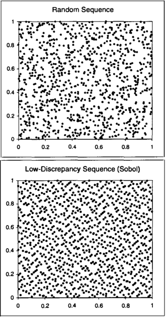
where the constant c(d) depends only on the problem dimension d. The idea behind the low-discrepancy se­ quences is to let the fraction of the points within any subset E of [0, 1]d of the form [0, vi ) x ... x [0, vd ) be as close as possible to its volume. That way, the low-discrepancy sequences will spread over [0, 1]d as uniformly as possible, reducing gaps and clustering of points. Figure 1 uses two-dimensional projection of a random sequence and of a low-discrepancy sequence to demonstrate the fundamental difference between the two classes of sequences.

Suppose we want to estimate I= Jro,I]d f(x)dx. Using

Monte Carlo sampling, we first generate a random se­ quence of independent vectors X1, x2, . .. , x N from the uniform distribution on [0, 1]d, then use 1J 2::�1 f(xi) as the estimator of I. The error bound for Monte Carlo sampling is probabilistic with order O(N- 1 1 2 ). In quasi-Monte Carlo methods, we use a low-discrepancy sequence x1, x2, ... , XN instead of a random se­ quence to estimate I. The integration accuracy for quasi-Monte Carlo methods relates to star discrepancy by the Koksma-Hlawka inequality (see [Niederreiter, 1992b])

where V (f) < oo is the variation of f in the sense of Hardy and Krause (see [Niederreiter, 1992b]). It is easy to see that with an increase in N quasi-Monte Carlo methods may offer better convergence rates than Monte Carlo sampling. Another advantage of quasi­ Monte Carlo methods is that we obtain deterministic error bounds 0( (log N)d IN).

Unfortunately, the theory has it that when the prob­ lem dimension d is high, it takes much larger N for the quasi-Monte Carlo methods to be superior over Monte Carlo sampling. For example, in a 20dimensional problem, (log N) 20 IN is still greater than 1IN 1 1 2 when N < 1075. This observation has con­ tributed to the belief that quasi-Monte Carlo methods are not effective in high-dimensional problems [Bratley et al., 1992, Morokoff and Caflisch, 1994]. However, several experimental tests [Paskov and Traub, 1995, Paskov, 1997, Papageorgiou and Traub, 1997] contra­ dicted this theoretical prediction and demonstrated that quasi-Monte Carlo methods can be very effective also in high-dimensional integral problems.

The basic low-discrepancy sequences proposed in the literature are those of Halton [1960], Sobol [1967], and Faure [1982]. Niederreiter [1992b] proposed a general principle for constructing so-called (t, d)-sequences. The sequences of Halton, Sobol and Faure can be viewed as special cases of generalized (t, d)-sequences.

3 Construction of Low-Discrepancy Sequences

In this section, we briefly describe the construction of three low-discrepancy sequences - Halton, Sobol and Faure sequences. General principles of generating low­ discrepancy sequences can be found in [Niederreiter, 1992b].

3.1 The Halton Sequence

Let p1, P2 , . . . , P d be the first d prime numbers. The Halton d-dimensional sequence [Halton, 1960] is de­ fined as sequence

where �Pi (n) is the jth radical inverse function:

This sum is finite with the integer coefficients a i (j, n) E [ O,p i - 1] (j and n are indexes) coming from the digit expansion of the integer n in base Pi

3.2 The Sobol Sequence

The Sobol sequence [1967] is generated from a set of special binary fractions of length w bits, vf, i = 1, 2, . .. , w, j = 1, 2, . . . , d. The numbers vf are called direction numbers.

In order to generate direction numbers for dimension j, we start with a primitive (irreducible) polynomial over the field F2 with elements { 0, 1}. Suppose the primitive polynomial in dimension j is

The direction numbers in dimension j are generated using the following q-term recurrence relation

where i > q. EB denotes the bitwise XOR operation. The initial numbers v{ · 2w, v � · 2w, . . . , v t · 2w can be arbitrary odd integers smaller than 2, 22, ... , and 2q, respectively. The Sobol sequence x� (n = L:�= O b i 2 i , b i E {0, 1}) in dimension j is generated by

We should use a different primitive polynomial to gen­ erate Sobol sequence in each dimension.

Antonov and Saleev [1979] proposed an efficient vari­ ant of Sobol sequence based on Gray code. An imple­ mentation of this variant is described in [Bratley and Fox, 1988].

3.3 The Faure Sequence

The Faure sequence [1982] can be generated as follows. Let p be the first prime number such that p � d and

pm is the upper bound of the sample size. Let C i j = (j) mod p, 0 :::; j :::; i :::; m. Consider the base p representation of n for n = 0, 1, 2, . . . ,

where a i (n ) E [ O , p ) are integers. The first coordinate of the point Xn is then given by

The other coordinates are given by

in order of i = 2, . . . , d. An algorithm for fast gen­ eration of Faure sequences could be found in [Tezuka, 1995].

Even though there exist other theoretical low­ discrepancy sequences with asymptotically good be­ havior (i.e., with small value of c(d)), such as Niederre­ iter sequence [Niederreiter, 1988] or Niederreiter-Xing sequence [Niederreiter and Xing, 1996], we will not dis­ cuss them here. Practical usability of these sequences requires careful testing and solving implementational issues. It is not certain that sequences with asymptot­ ically good behavior will necessarily perform well in practical applications, where only a finite number of points near the beginning of the sequence are used.

4 Quasi-Monte Carlo Methods m Bayesian Networks

In this section, we describe our adaptation of quasi­ Monte Carlo algorithms to belief updating in Bayesian networks. We focus on importance sampling algo­ rithms, currently the best performing stochastic sam­ pling algorithms (see [Cheng and Druzdzel, 2000]). We start with a brief general description of sampling algo­ rithms and follow this by a description of importance sampling. Finally we propose an algorithm for gener­ ation of direction numbers in Sobol sequence.

4.1 Stochastic Sampling in Bayesian Networks

We know that the joint probability distribution over all variables of a Bayesian network model, Pr(X), is the product of the probability distributions over each of the nodes conditional on their parents, i.e.,

In order to calculate the probability of evidence Pr(E = e), we need to sum over all Pr(X\E, E =e),

The posterior probability Pr(aJe) can be obtained by first computing Pr( a, e) and Pr( e) separately accord­ ing to equation (2), and then combining these two based on the definition of conditional probability

Stochastic sampling algorithms attempt to obtain an estimate of Pr(E = e) in equation (2), which is anal­ ogous to approximate computation of integrals. The number of summation terms, which we will denote by d(X\E), corresponds to the dimension of the problem.

In order to estimate Pr(E = e), we can first gener­ ate a low-discrepancy sequence of x1 , x2, ... , x N in d(X\E) dimension unit supercube using the methods described in Section 3. Every dimension j corresponds to a node in X\E. Then the value x { can be processed as a random number generated for the corresponding node in sample i. Using this conversion method, low­ discrepancy sequences can be easily applied to many sampling algorithms, such as probabilistic logic sam­ pling [Henrion, 1988], likelihood weighting [Fung and Chang, 1989, Shachter and Peat, 1989], importance sampling [Shachter and Peat, 1989], or AIS-BN sam­ pling [Cheng and Druzdzel, 2000].

4.2 Importance Sampling for Bayesian Networks

Sampling algorithms will in general work very well when the estimated function Pr(X\E, E =e) is smooth. When Pr(X\E, E =e) is not smooth, the performance of sampling algorithms will deteriorate (i.e., their convergence rate will be very slow). This is also true for quasi-Monte Carlo methods. Impor­ tance sampling algorithms [Shachter and Peot, 1989, Cheng and Druzdzel, 2000] address this problem by choosing an appropriate sampling distribution. The main principle of importance sampling can be sum­ marized as an attempt to find an importance density sampling function Pr isf (X\E) that will let

be as smooth as possible. Another requirement for the importance sampling function Pr isf (X\E) is that it should be easy to generate samples according to that function. If we generate samples x1, x2, ... , XN ac­ cording to the function Pr isf (X\E) independently and

randomly, then f:t 2:�1 f( x; ) is an unbiased estimator of Pr(E = e). A thorough discussions of detail of im­ portance sampling in Bayesian networks can be found in [Cheng and Druzdzel, 2000).

4.3 Direction Numbers in Sobol Sequence

Suppose that we choose a primitive polynomial of de­ gree q that will generate Sobol sequence in a certain di­ mension. From the discussion in Section 3.2, we know that the initial numbers v { · 2w, v 4 · 2w, .. . , v t · 2w in Sobol sequence can be arbitrary odd integers smaller than 2, 22, · · · , 2q respectively. A simple calculation shows that there are a total of 2q·(q-l}/2 ways of choos­ ing these q integers. For dimension of 36 (in which case q has to be 8 or higher), this number is larger than 227. Considering all dimensions makes the total space for the initial direction numbers huge. We have found experimentally that the choice of these numbers affects the convergence rate significantly. Although Paskov and Traub [ 1995) and Paskov [1997) mention that they made improvements in the initial direction numbers for the Sobol sequence, they do not reveal the method that they used. This section proposes an al­ gorithm for the choice of initial direction numbers for quasi-Monte Carlo methods in Bayesian networks.

Since the idea behind the low-discrepancy sequences is to let the points be distributed as uniformly as possi­ ble, we introduce an additional measure of uniformity of the distribution of a set of points that will be useful in choosing direction numbers. Essentially, to compute this measure of uniformity, we divide the unit square into m2 equal parts. Ideally, each part should have N jm2 points. We calculate the sum of the absolute differences between the actual and the ideal number of points in each part. This measure is heuristic in nature, as it looks at only two dimensions at a time. We have found empirically that the direction numbers based on this uniformity property are reasonable.

Suppose that we have obtained the initial direction numbers for the first i dimensions and have derived the first N points x { , j = 1, 2, ... , i , l = 1, 2, ... , N, based on these numbers. For the dimension i + 1, we randomly choose the initial numbers v f +1 · 2w, v � +l · 2w, .. . , v � +l · 2w and then calculate x ; +l, l = 1, 2, ... , N. After computing the sum of the uniformity discrepancy in the unit square given by dimensions i + 1 and each of the i dimensions based on these N points, we choose the initial direction numbers that minimize the sum as our initial direction numbers in dimension i + 1. This is essentially a random search process. (Due to the size of the search space, it is impossible to conduct an exhaustive search.) Figure 2 contains an algorithm describing our approach.

for i +1 to nDimension do for j +-1 to nRandom Times do Randomly choose the initial direction numbers for dimension i S;(N) +Get the first N Sobol sequence in dimension i according to previously chosen initial direction numbers nErrorSum+0 for k +1 to i -1 do nError+Calculate the uniformity discrepancy in the unit square given by dimensions k and i based on Sk(N) and S;(N) nErrorSum+- nErrorSum+w(k, i)·nError end for keep the best initial direction numbers and corresponding S;(N) so far based on nErrorSum end for end for

We know that in Bayesian networks parent nodes af­ fect their children directly. A good sampling heuristic is to keep parent nodes close to their children in the sampling order and to keep those dimensions that are close together more uniformly distributed. We achieve this by giving a higher weight w(k, i) to those dimen­ sions that are close to each other when computing the uniformity discrepancy. In our tests, we have chosen N = 1 , 02 4 , m = 32 and w(k,i) = 1 when k 2': i 8, otherwise w(k, i) = 0.

5 Experimental Results

We performed empirical tests comparing Monte Carlo sampling to quasi-Monte Carlo methods using five net­ works: COMA [Cooper, 1984), As i A [Lauritzen and Spiegelhalter, 1988), ALARM [Beinlich et al., 1989), HAILFINDER [Abramson et al ., 1996, Edwards, 1998), and a simplified version of the CPCS (Computer­ based Patient Case Study) network [Pradhan et al., 1994]. The first four networks can be downloaded from http://www2.sis.pitt.edu/.....,genie. The CPCS network can be obtained from the Office of Technol­ ogy Management, University of Pittsburgh. Each of the tested networks is multiply-connected and the last three networks are multi-layer networks with multi­ valued nodes. In case of the CPCS network, we have used the largest available version for which comput­ ing the exact solution is still feasible, so that we could compute the approximation error in our experiments. The sizes of the networks (this corresponds directly to the dimension of the sampling space) ranged from 5 to 179. Each of these networks has been used in

the UAI literature for the purpose of demonstration or algorithm testing. Most of them are real or realistic with both the structure and the parameters elicited from experts. We believe that our test set was quite representative for practical networks.

We focused our tests on the relationship between the number of samples and the accuracy of approximation achieved by the simulation. We measured the latter in terms of the Mean Square Error (MSE), i.e., square root of the sum of square differences between Pr' (Xij) and Pr(Xij), the sampled and the exact marginal prob­ abilities of state j (j = 1, 2, . . . , ni) of node i , such that Xi rf. E. More precisely,

where X is the set of all nodes, E is the set of evidence nodes, and ni is the number of outcomes of node i . In all diagrams, the reported MSE for Monte Carlo sampling is averaged over 10 runs. Since quasi-Monte Carlo methods are deterministic, we report MSE of a single run.

We varied the number of samples from 250 to 256, 000, staring at 250 and doubling this number at each of the subsequent 10 steps (yielding a total of 11 sampling steps in each test). In all figures included in this paper, we show plots of log1 0 MSE against log2 (N /250), where N is the number of samples. We connect the points in the plots by lines in order to indicate the trend. The linear behavior observed in the log-log plots cor­ responds to a relationship MSE= eN-a., where a can be estimated by means of linear regression. For Monte Carlo sampling, the theoretical value of a is 0.5.

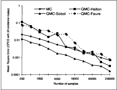
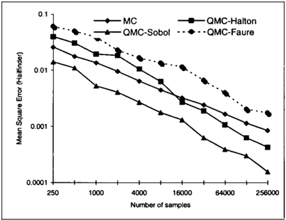
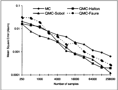
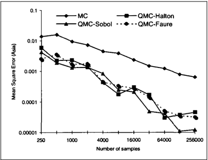
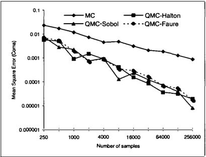
Our first tests involved belief updating without evi­ dence. In this case, we used the probabilistic logic sampling algorithm [Henrion, 1988]. The results are shown in Figures 3 through 7. The estimated values of a for different networks and different sampling meth­ ods are shown in Table 1. The results of tests for low­ dimensionality problems (Figures 3 and 4) show that the three quasi-Monte Carlo methods tested are sig­ nificantly better than Monte Carlo sampling. The dif­ ferences among the three quasi-Monte Carlo methods are small. For a given sample size, such as 8, 000, the smallest improvement of MSE is larger than 1,100% (one order of magnitude). The accuracy achieved by Monte Carlo sampling with 256, 000 samples will be achieved by the quasi-Monte Carlo methods with only 4, 000 sample points (two orders of magnitude less). With the increase of the problem dimension, the results change. The accuracy achieved by means of Faure and Halton sequences deteriorates. For the

HAILFINDER and CPCS networks, the Faure sequence leads to performance that is even worse than that of Monte Carlo sampling. Although the method using Halton sequence is worse than Monte Carlo sampling when the sample size is small, its convergence rate a (Table 1) is better than that of Monte Carlo sampling ( a = 0.5) and when the sample size is large enough, the Halton sequence catches up. As the number of di­ mensions increases, the accuracy of the Sobol sequence appears to be better than that of the other two quasi­ Monte Carlo methods. A remarkable result is that the method using Sobol sequence is significantly better than Monte Carlo sampling in all five tested networks. In the CPCS network, for a given sample size, such as 8, 000, the improvement of MSE is 372% (almost an order of magnitude). The accuracy achieved using

256, 000 sample points by Monte Carlo sampling will required about 16, 000 sample points in the method using Sobol sequence (still over an order of magnitude improvement). Its convergence rate a = 0.71 is also better than that of Monte Carlo sampling ( a = 0.5), which means that higher number of samples will lead to even larger improvement. Table 1 shows that the convergence rate a of quasi-Monte Carlo methods was always better than Monte Carlo sampling. It seems that the method using Halton sequence leads to bet­ ter convergence rates than that using Faure sequence with the increase of dimensions.

Table 1: Estimated convergence rates a for the six test cases and four tested sampling methods. CPCS/E stands for the CPCS network with 20 evidence nodes.

a	MC	Halton	Sobol	Faure
COMA	0.46	0.87	0.88	0.82
A S IA	0.49	0.76	0.90	0.74
ALARM	0.51	0.74	0.65	0.72
HAILFINDER	0.50	0.69	0.64	0.53
CPCS	0.51	0.74	0.71	0.57
CPCS/E	0.50	0.82	0.61	0.70

Our final test focused on evidential reasoning. As men­ tioned before, in evidential reasoning, when the func­ tion Pr(X\E, E = e ) is not smooth, the performance of sampling methods will in general be poor. In or­ der to compare Monte Carlo sampling to quasi-Monte Carlo methods, we based our tests on the adaptive importance sampling algorithm (AIS-BN) developed in our earlier work [Cheng and Druzdzel, 2000]. The AIS-BN algorithm first learns the optimal importance sampling function by adjusting dynamically equation

(3). In our earlier tests involving evidential reasoning with very unlikely evidence, the AIS-BN algorithm has consistently outperformed the likelihood weighting al­ gorithm by several orders of magnitude. As the focus of the current paper is a comparison of Monte Carlo sampling to quasi-Monte Carlo methods, we used the same importance sampling for both. We run the AIS­ BN algorithm until it has found a good importance function Pr isf (X\E) and then used importance sam­ pling (Section 4.2) to compare Monte Carlo sampling to quasi-Monte Carlo methods. We used only the CPCS network in our tests, as it has observable nodes indicated as such. Our test cases for evidential reason­ ing were, therefore, quite realistic. Figure 8 shows a

typical plot of convergence. The plot shows that the Sobol sequence leads to the best results, similarly to the results of our tests without evidence. For example, for the sample size of 8,000, the improvement of the Sobol sequence over Monte Carlo sampling is 293%. The accuracy achieved by 256,000 sample points in Monte Carlo sampling would require less than 32, 000 sample points using Sobol sequence (over an order of magnitude improvement in speed over Monte Carlo sampling). Its convergence rate o: = 0.61 is better than that of Monte Carlo sampling ( o: = 0.5). The behavior of Halton and Faure sequences is almost the same as without evidence. It is worth to point out that the improvement using Sobol sequence depends on the smoothness of the function f(X\E)- the more smooth the function is, the higher the improvement.

Quasi-Monte Carlo methods preserve the anytime property of sampling algorithms. All plots of our ex­ perimental results indicate that the convergence curve of the Sobol sequence is quite smooth. It is fairly safe to terminate the simulation at any time and still ob­ tain a reasonable result. This is different from Monte Carlo sampling, which is sensitive to the random seed and often shows large variance (please note that our plots of Monte Carlo sampling performance are smooth because they are averaged over 10 runs).

With an increase in problem dimension, one of the threats to accuracy is a possible significant correla­ tion between different dimension in low-discrepancy sequences. The algorithm we used to select the direc­ tion numbers for the Sobol sequence tries to decrease this correlation. Other methods that aim at decreas­ ing this correlation and improve the low-discrepancy sequences can be found in [Kocis and Whiten, 1997]. Although their methods are reported to reduce the er­ ror variance, we did not see significant improvement in our tests.

Currently, there exists no general rigorous theoreti­ cal justification that would explain why quasi-Monte Carlo methods are superior to Monte Carlo sampling across the variety of application studied. Several rea­ sonable explanations have been proposed. Caflisch, Morokoff and Owen [1997] suggest that quasi-Monte Carlo methods are superior to Monte Carlo sam­ pling if the effective dimension of the integrand is not large. Another explanation is that the error bounds O((Iog N) d j N) in quasi-Monte Carlo meth­ ods are of the order of the upper bounds given by the inequality which can be a very loose inequality for a particular function. Since the inequality (1) is very conservative and calculating V(f) is difficult, us­ ing inequality (1) to estimate the error is not prac­ tical. There are some papers (e.g., [Owen, 1995, Kocis and Whiten, 1997]) discussing the error estima­ tion in quasi-Monte Carlo methods.

In terms of absolute computation time, we have ob­ served that generation of one Sobol and one Faure point takes respectively about 57% and 29% less than generation of one random sample. As a complete sam­ pling algorithm consists of other steps that are the same for Monte Carlo and quasi-Monte Carlo algo­ rithms, the effective difference in computation time is smaller. We would like to caution the reader that these comparisons are implementation-dependent and an efficient algorithms for generating low-discrepancy sequences or random numbers can change these re­ sults.

6 Conclusion

Quasi-Monte Carlo methods can significantly improve the performance of sampling algorithms in Bayesian networks. In our tests, as the number of dimensions increased, the sampling method using Sobol sequence outperformed the methods using Halton and Faure sequences. Compared to Monte Carlo sampling, the quasi-Monte Carlo approach using Sobol sequence not only had a better start coefficient, but also had a bet­ ter convergence rate. The exact improvement in per­ formance depends on the smoothness of the sampling function. In sampling without evidence, we observed as much as a 3.5-fold improvement in the Mean Square Error. For a fixed level of the Mean Square Error, we observed more than a 15-fold decrease in sampling time. Given their consistently better performance over

Monte Carlo sampling, we expect that quasi-Monte Carlo methods will be widely applied in Bayesian net­ work inference.

We also believe that approximate inference in Bayesian networks is an excellent test bed for studying the prop­ erties of low-discrepancy sequences. There is a multi­ tude of test data and extending the problem dimension is natural. ·

Acknowledgments

This research was supported by the National Science Foundation under Faculty Early Career Development (CAREER) Program, grant IRI-9624629, and by the Air Force Office of Scientific Research under grants F49620-97-1-0225 and F49620-00-1-0112. Malcolm Pradhan and Max Henrion of the Institute for De­ cision Systems Research shared with us the CPCS network with a kind permission from the developers of the Internist system at the University of Pitts­ burgh. Anonymous reviewers provided us with use­ ful suggestions for improving the clarify of the pa­ per. All experimental data have been obtained us­ ing SMILE, a Bayesian inference engine developed at the Decision Systems Laboratory and available at http://www2.sis.pitt.edu/�genie.

References

[Abramson et al., 1996]

Bruce Abramson, John Brown, Ward Edwards, Al­ lan Murphy, and Robert Winkler. Bayesian pre­ diction of severe weather. International Journal of Forecasting, 12(1):57-71, March 1996.

[Antonov and Saleev, 1979] I. A. Antonov and V. M. Saleev. An economic method of computing lpr sequences. U.S.S.R. Computational Mathematics and Mathematical Physics, 19:252-256, 1979.

[Beinlich et al., 1989] I.A. Beinlich, H.J. Suermondt, R.M. Chavez, and G.F. Cooper. The ALARM mon­ itoring system: A case study with two probabilistic inference techniques for belief networks. In Proceed­ ings of the Second European Conference on Arti­ ficial Intelligence in Medical Care, pages 247-256, London, 1989.

[Bratley and Fox, 1988] Paul Bratley and Bennett L. Fox. Algorithm 659 : Implementing Sobol's quasir­ andom sequence generator. ACM Transactions on Mathematical Software, 14(1):88-100, 1988.

[Bratley et al., 1992] Paul Bratley, Bennett L. Fox, and Harald Niederreiter. Implementation and tests of low-discrepancy sequences. ACM Transaction on

Modeling and Computer Simulation, 2(3):195-213, 1992.

[Caflisch et al., 1997] Russel E. Caflisch, William J. Morokoff, and Art B. Owen. Valuation of mortgage backed securities using Brownian bridges to reduce effective dimension. Journal of Computational Fi­ nance, 1:27-46, 1997.

[Cheng and Druzdzel, 2000] Jian Cheng and Marek J. Druzdzel. AIS-BN: An adaptive importance sam­ pling algorithm for evidential reasoning in large Bayesian networks. Under review, 2000.

[Cooper, 1984] Gregory F. Cooper. NESTOR: A Computer-based Medical Diagnostic Aid that Inte­ grates Causal and Probabilistic Knowledge . PhD thesis, Stanford University, Computer Science De­ partment, 1984.

[ Cooper, 1990] Gregory F. Cooper. The computa­ tional complexity of probabilistic inference using Bayesian belief networks. Artificial Intelligence, 42(2-3):393-405, March 1990.

[Edwards, 1998] W. Edwards. Hailfinder: Tools for and experiences with Bayesian normative modeling. American Psychologist, 53:416-428, 1998.

[Faure, 1982] H. Faure. Discrepance de suites asso­ ciees a un systeme de numeration (en dimension s). Acta Arithmetica, 41:337-351, 1982.

[Fung and Chang, 1989] Robert Fung and Kuo-Chu Chang. Weighing and integrating evidence for stochastic simulation in Bayesian networks. In Un­ certainty in Artificial Intelligence 5, pages 209-219, New York, N. Y., 1989. Elsevier Science Publishing Company, Inc.

[Halton, 1960] J. H. Halton. On the efficiency of cer­ tain quasirandom sequences of points in evaluat­ ing multidimensional integrals. Numerische Mathe­ matik, 2:84-90, 1960.

[Henrion, 1988] Max Henrion. Propagating uncer­ tainty in Bayesian networks by probabilistic logic sampling. In Uncertainty in Artificial Intellgience 2, pages 149-163, New York, N.Y., 1988. Elsevier Sci­ ence Publishing Company, Inc.

[Kocis and Whiten, 1997] Ladislav Kocis and William J. Whiten. Computational investigations of low-discrepancy sequences. ACM Transactions on Mathematical Software, 23(2):266-294, 1997.

[Lauritzen and Spiegelhalter, 1988] Steffen L. Lau­ ritzen and David J. Spiegelhalter. Local computa­ tions with probabilities on graphical structures and

• their application to expert systems. Journal of the Royal Statistical Society, Series B (Methodological), 50(2):157-224, 1988.
• [Morokoff and Caflisch, 1994] William J. Morokoff and Russel E. Caflisch. Quasi-random sequences and their discrepancies. SIAM Journal on Scien­ tific Computing, 15(6):1251-1279, 1994.
• [Morokoff and Caflisch, 1995] William J. Morokoff and Russel E. Caflisch. Quasi-Monte Carlo integra­ tion. Journal of Computational Physics, 122:218230, 1995.
• [Niederreiter and Xing, 1996] Harald Niederreiter and Chaoping Xing. Low-discrepancy sequences and global function fields with many rational places. Fi­ nite Fields and Their Applications, 2:241-273, 1996.
• [Niederreiter, 1988] Harald Niederreiter. discrepancy and low-dispersion sequences. of Number Theory, 30:51-70, 1988. Low­ Journal
• [Niederreiter, 1992a] Harald Niederreiter. Quasiran­ dom sampling computer graphics. In Proceedings of the 3rd International Seminar on Digital Image Processing in Medicine, pages 29-33, 1992.
• [Niederreiter, 1992b] Harald Niederreiter. Random Number Generation and Quasi-Monte Carlo Meth­ ods. SIAM, CBMS-NSF Regional Conference Series in Applied Mathematics, Number 63, 1992.
• [Owen, 1995] Art B. Owen. Randomly permuted (t, m, s)-nets and (t, s)-sequences. In H. Niederre­ iter and P. J.-S. Shiue, editors, Monte Carlo and Quasi-Monte Carlo Methods in Scientific Comput­ ing, pages 299-317. Springer-Verlag, New York, 1995.
• [Papageorgiou and Traub, 1997] Anargyros Papageorgiou and Joseph F. Traub. Faster evalu­ ation of multidimensional integrals. Computers in Physics, 11(6):574-579, 1997.
• [Paskov and Traub, 1995] Spassimir H. Paskov and Joseph F. Traub. Faster valuation of financial derivatives. Journal of Portfolio management, Fall:113-120, 1995.
• [Paskov, 1997] Spassimir H. Paskov. New method­ ologies for valuing derivatives. In S. Pliska and M. Dempster, editors, Mathematics of Derivative Securities, pages 545-582. Cambridge University Press, 1997.
• [Pradhan et al., 1994] Malcolm Pradhan, Gregory Provan, Blackford Middleton, and Max Henrion. Knowledge engineering for large belief networks. In
• Proceedings of the Tenth Annual Conference on Un­ certainty in Artificial Intelligence (UAI-g4), pages 484-490, San Francisco, CA, 1994. Morgan Kauf­ mann Publishers.

[Shachter and Peot, 1989] Ross D. Shachter and Mark A. Peot. Simulation approaches to general probabilistic inference on belief networks. In Un­ certainty in Artificial Intelligence 5, pages 221-231, New York, N. Y., 1989. Elsevier Science Publishing Company, Inc.

• [Sobol, 1967] I. M. Sobol. On the distribution of points in a cube and the approximate evaluation of integrals. U.S.S.R. Computational Mathematics and Mathematical Physics, 7(4):86-112, 1967.
• [Tezuka, 1995] Shu Tezuka. Uniform Random Num­ bers: Theory and Practice. Kluwer Academic Pub­ lishers, Boston, 1995.