Contents
1302.3550
Constraining Influence Diagram Structure by Generative Planning: An Application to the Optimization of Oil Spill Response
John M. Agosta SRI International 333 Ravenswood A venue Menlo Park, CA 94025 j ohnmark<Dsri . com
Abstract
tice of decision analysis as an alternate representation for trees.
This paper works through the optimization of a real world planning problem, with a com bination of a generative planning tool and an influence diagram solver. The problem is taken from an existing application in the do main of oil The planning agent manages constraints that or der sets of feasible equipment employment actions. This is mapped at an intermedi ate level of abstraction onto an influence di agram. In addition, the planner can apply a surveillance operator that determines observ ability of the state-the unknown trajectory of the oil. The uncertain world state and the objective function properties are part of the influence diagram structure, but not repre sented in the planning agent domain. By ex ploiting this structure under the constraints generated by the planning agent, the influ ence diagram solution complexity simplifies considerably, and an optimum solution to the employment problem based on the objective function is found. Finding this optimum is equivalent to the simultaneous evaluation of a range of plans. This result is an example of bounded optimality, within the limitations of this hybrid generative planner and influence diagram architecture.
1 Introduction
Determining which actions to take and when has been addressed by distinct methods in AI. Among them are two techniques that choose actions in sequence to meet a specified goaL One is generative planning, coming out of the classical planning field; and the other, influ ence diagrams, out of the methods of Bayesian proba bility. Classical planning has its origins in symbolic reasoning methods created to address difficulties in conventional logic as facts change over time. Influence diagrams are Bayes' networks with decision and value nodes added, which were first introduced in the prac-
There have been attempts to find a sound extension of classical AI planning that encompasses uncertainty, or vice versa, to develop a decision theoretic plan ning method that structures the decision basis in ad dition to determining the best policies. Either ex tension must deal with the combinatorial complex ity of generative planning on top of the complexity of the uncertainty calculation. (Blythe 1996] [Draper, Hanks and Weld 1994][Haddawy, Doan and Goodwin 1 995][Lehner, Elaesser and Mus man 1994][Lowrance and Wilkins 1990] The line of work presented here has a more modest goal; to demonstrate that the com bination of planning and influence diagram methods can simplify the computational complexity of a real world problem by orders of magnitude. This solution exploits the abilities of the generative planner to man age constraints among sets of actions and the influence diagram to indicate irrelevant structure from the com binations of available actions, uncertainties and the objective function. The computational example pre sented in this paper suggests how the two methods in combination constitute an architecture for solution of complicated problems by working through a solution to an oil spill emergency response problem. On the one hand, the constraints generated by the planning agent determine the order and the range of actions in corporated in the structure that the influence diagram uses for optimization. On the other hand, the rich ness of the the influence diagram model can focus on which uncertainties and sets of actions are relevant, to further constrain the search of an optimum.
Beyond the practical value of this approach in solv ing real-world problems, this work has value in ex ploring the insight that as problems become more un certain, the complexity of the planning problem can decrease rather than increase. The basis of this in sight comes from the practice of modeling complex, un certain problems in decision analysis, where the com putational complexity of the models employed tends to be small. Decision analysis exploits properties of dominance and value of information, so that the model structure or computation generating informa-
tion found to be irrelevant to the problem can be pruned.
My approach addresses similar concerns to methods of plan evaluation, in its ability to rank the quality of plans that have been generated by a planning agent. The term "plan evaluation" can also refer to measuring the success and computational performance of plan ning agents. A method that has been developed for plan evaluation in the first sense, called action net works [Goldszmidt and Darwiche 1994], has a strong similarity to the method applied in this paper. In con trast to action networks, influence diagrams represent decisions prior to deliberation and serve to optimize the choices at decisions. This also makes them capa ble of pre-posterior analysis, exploited in this paper, such as the computation of value of information, of which action networks are not capable. Of course, the lessons learned from action networks about represent ing time and persistence still apply.
The rest of this section reviews the model domain and architecture. Section 2 is a short summary of stochas tic optimization. The step by step transformation and solution of the problem occupies Section 3, followed by conclusions in Section 4.
1.1 The U.S. Coast Guard Oil Spill Response Configuration System
We have developed a planning tool under contract with the U.S. Coast Guard (USCG) to assist them in the al location and siting of the equipment available to clean up anticipated oil spills. As part of their required pre paredness planning, the Spill Response Configuration System (SRCS) assists in determining the adequacy of the equipment to meet the threat of spills; for in stance, either to determine to purchase more equip ment, or, for that already staged at storage sites near the coast, to determine where best to site it. SRCS meets this objective by building plans against simu lated oil spills to estimate the effectiveness of USCG's ability to clean them up. As intended in the origi nal design, SRCS uses a generative planning tool, Sys tem for Interactive Planning and Execution (SIPE-2) [Wilkins 1988], to guide the user interactively through a set of progressively more detailed choices, first to choose cleanup strategies and then allocate and em ploy equipment against a chosen spill scenario. This paper describes an extension to SRCS to evaluate a range of plans generated by SIPE-2, and to choose the best.
1.2 The Agent Architecture
One approach to the limits that computation places on rational choice is to begin with a computational architecture-in this case a hybrid of two techniques and optimize the solution method within the con straint of these architectural limitations on informa tional and computational resources. This extends the idea of "heuristic adequacy." Rather than beginning with the concept of a purely rational agent, and by approximation, whittling it down to make it tractable, this approach, termed bounded optimality, begins with the architectural assumption. Arguments for this ap proach to AI research, first made by Horvitz, are ex� panded in Russell's invited paper at the last IJCAI. [ Russell 1995]
We may characterize a rational architecture by what computational and sensing abilities it possesses:
- generative/evaluative: How much can the agent structure the problem?
- static/dynamic: Can it reason about changes over time?
- unobservable/ observable: Is the state of the world accessible to the agent when it chooses?
- deterministic/uncertain: Can it reason with par tial or incomplete knowledge?
- episodic/continuous control: Can it intervene only at selected times?
- discrete actions/ continuous actions: Is the range of actions at any time finite or continuously vari able?
In this application, generative planning is generative, dynamic, unobservable, deterministic, episodic and discrete. Influence diagrams are evaluative, dynamic, observable, uncertain, episodic and discrete. The com� bination includes three differences: generative versus evaluative, unobservable versus observable and deter ministic versus uncertain. The comparison is perhaps unfair; the two methods purport to do different things. In generative planning, actions are distinguished by simply whether or not they achieve a goal, rather than the degree to which they achieve an objective. In com parison influence diagrams need to consider the degree of achievement of an objective to be able to optimize.
In looking to combine these methods I have taken a practical approach, asking which outputs of a mature planning tool, e.g. SIPE-2 can be used to structure an influence diagram that can then optimize the prob lem. As a stochastic optimization technique, influence diagrams solve a class of decision under uncertainty problems based on a quantitative objective, however the input to an influence diagram solver is a structure that has already determined the set of allowed actions and information observable in each episode, and the ordering of decision episodes. The challenge then, is to what extent can a generative planning tool create this linear ordering for the influence diagram, which I will call the decision backbone.
In the least commitment philosophy adopted by gen erative planning, the planning agent approaches the problem by a top down successive refinement method, terminating when the problem has been reduced to the lowest level procedures represented in its knowl edge base. As the plan is refined, actions that pre-
viously were parallel tend to become ordered. The process adds constraints to the set of actions, both by sequencing them in time, and by restricting the set of actions available at any one time. The process may be non-deterministic, in that if the problem is not fully constrained, the planner might arrive at any one of a number of satisfactory plans that meets the planning goals. In this work I don't examine exactly how the planner generates the plan; instead I examine which information is available to the planner, and how its constraints can be interpreted to structure the influ ence diagram for the problem. The answer in short, is first to use the planner output to sequence decisions in the influence diagram, and second to constrain sets of available actions at each decision point in the in fluence diagram. If the ordering of actions and the observations available at each set of actions are com pletely ordered, then the result is a single influence diagram. Actions to observe uncertain states are not typically encoded in a planner's set of operators al though they are needed in the design of an influence diagram. To demonstrate the consequences of observa tions in a plan, the oil spill example has a surveillance operator that generates an observation action for the uncertain trajectory state.
In generative planning, refinement steps generate lev els of the plan hierarchy that vary in their level of abstraction. As the planning agent applies operators to goals at one level, they are expanded into sub-plans at lower levels. It has been recognized that the ability to work at varying levels of abstraction offers a ma jor simplification to the search problem. In contrast, the influence diagram works entirely at one level of ab straction. It is not my intent to make a contribution to the theory of abstraction per se, but, as with other features of generative planning, to show how abstrac tion can be exploited. The key to this is to recognize, at each decision point, which level of abstraction in the plan should be represented in the influence diagram.
This design decision depends on the level of the actions that have the most direct relevance to variables in the objective function, i.e.-that most directly correspond to the quantities of which the objective is a function. In this model these are the quantities of equipment employed in a sector. Other levels of the planning agent's goal-expansion operators are relevant to the objective only in how they constrain actions at the relevant leveL They do not have a direct effect on the objective.
1.3 Concepts of value and goal achievement
The similarity between the notion of planning to meet a goal and of optimizing to improve an objective func tion hides the fact that they are represented differ ently, and serve different purposes in this architecture. A goal represents achievement of a binary condition; an objective represents a complete ordering of out comes. (For an extended discussion on this see [Dean and Wellman 1991] section 5.6.) On the kind of prob lems with which classical planning started out, a bi nary condition as an objective is appropriate. These problems have all or nothing solutions, like jumping a chasm, or tossing a bean bag into a box. The value of the objective is high and constant if the bag falls in the box, or the chasm is breached, but low otherwise.
In this application, the planning goals and the objec tive function are used for different purposes in the ar chitecture. The objective function of SRCS to be min imized is the expected quantity of oil that reaches the shore. Equivalently, this can be expressed as mini mizing the fraction of oil that reaches the shore out of the total amount that would reach the shore if no actions were taken. The rich physical domain model expressed in the objective function that the optimiza tion routine applies has no counterpart in the domain model of the planning agent. Even if there were a sat isfactory way to dichotomize the objective outcomes into achievement and failure of a goal, this would not serve the purpose of using the planner to constrain the action sets of the influence diagram optimization. Instead, the planning goals represent the achievement of feasible actions to locate and transport equipment, at different levels of abstraction. The planning agent finds sets of actions that meet these goals, by consider ing, for example, what combinations of equipment are either possible or necessary at each location, what con ditions were necessary before the equipment is brought to the location, or employed there, and what interac tions, both helpful and harmful might exist between actions. The planner is underconstrained so that there exist many plans that meet these goals within the plan ning constraints. Optimization then takes place within this feasible set of actions that the planner has so de termined.
2 Optimization under uncertainty
The general form of a stochastic optimization problem can be written:
where P( o) is a policy function of the subset, o, that can be observed of variables :r, and V() is a value function to be minimized. The world model is ex pressed as a joint distribution over all uncertain vari ables, pr{ x 10, where � is the decision maker's state of knowledge before the first decision is made. In general P(o) can be quite complicated. It can include a se quence of i episodes, each containing a decision, where generally E; for each decision includes all observations and choices made in previous episodes. This set of decisions is represented by a completely ordered set of nodes, called the decision backbone of the influence diagram.
Decisions occur episodically at times called decision
points. At each decision point where the entire cur rent state is observed, the problem can be factored, so that it can be solved in stages, and the policy at each stage is only a function of the current observed state. [Bertsekas 1987] This is shown in an influence diagram by a decision node, that, if removed-together with its uncertain direct predecessors-would split the decision backbone and disconnect the influence diagram net work. The resulting solution is a recurrence equation over return functions V; known as Bellman's equation:
It can be applied sequentially, starting with the last stage, with Vr set equal to the objective function, to solve the stochastic optimization problem, obtaining V* = V0. The complexity of this sequentially decom posable problem depends upon the size of the state space, �;, of each stage. This can still be large. For instance, in the oil spill problem this state space must describe the two dimensional distribution of the oil slick at a point in time.
Bellman's equation applies to the solution of influence diagrams whose decisions meet the observability con dition. To exploit this simplification, we will design structures where this condition occurs.
3 Solution of the best policy in the oilspill domain
3.1 The Nature of an Oil Spill Response
The problem addressed by SRCS is the emergency re sponse to large oil spills caused by the foundering of commercial tankers or barges that transport of oil. Typically such a spill involves thousands of barrels of oil released over t he course of several hours or days. The USCG and commercial carriers maintain on-call extensive inventories of oil spill response equipment in locations near ports where oil transport occurs. The expense to maintain this capability is small in com parison to the expected costs of damage and cleanup should a large spill reach shore.
By its nature, the oil spill cleanup problem is a race against time where the expanding extent of the threat due to the spreading oil slick is uncertain. The oil is dispersed by wind and tide in addition to advective spreading over the surface of the water. The purpose of the response is to prevent the oil from reaching sen sitive areas on the shore by use of floating containment booms and removal methods such as oil skimmers, dis persant chemicals, or controlled burning.
The response problem is to determine which equip ment should be dispatched when and where. Actions tend to concentrate 1) around the foundered ship, to prevent open water releases, 2) in open water, to re move the oil slick, and 3) at the shoreline, to protect sensitive areas. This categorization matches the high est level of abstraction of the planning operators. In this example we will restrict the actions considered to the use of booms and dispersants, without much loss of generality. For a specific incident, the location and weather often make it difficult to entirely control a spill discharge: Even with an optimal plan in this case the degree of containment and cleanup may be small. A detailed description of our formulation of this problem can be found in [ Desimone and Agosta 1994].
3.2 Derivation of the Architecture: The Approach to Simplifying the Model
This section addresses the simplifications possible to the model based on the architecture of the planning and optimization tools. A somewhat extreme ap proach was taken here, more as a demonstration of what kind of transformations are possible by exploit ing this hybrid architecture. Interestingly, within the bounds of the architecture, the optimality of the so lution obtained is not significantly compromised. The only concession to simplifying assumptions made in the model was to reduce the number of sensitive areas threatened to 3, down from 6.
3.2.1 Modeling of Trajectory Uncertainty
By borrowing from the modeling techniques used for oil trajectory modeling, [Spaulding 1988] significant reductions can be made in the size of the proba bility state space of the influence diagram. At the most general level, the dispersion of oil is a time dependent probability distribution of the amount of oil, q, over the two dimensional surface of the wa ter: pr{qju1,u2,t}. There are two common simplifi cations to this, by using either a Lagrangian frame or a Eulerian frame for discretization. In the Lagrangian formulation, which is standard practice for determin istic forecasting models, the quantity of spilled oil is discretized into "spillets" and each spillet 's trajectory is forecast. Then spillets in an area are averaged to estimate oil quantities at each location. In compar ison, in the Eulerian formulation, locations are dis cretized, and the quantities of oil are forecast on this grid. The disadvantage of the Eulerian formulation is that a diffusion process will propagate an infinitesimal quantity to each location, making it difficult to sim plify the computation by localizing it. We show the compensating advantage to the Eulerian formulation when uncertainty is considered is that the geographic discretization can be coarse, so the state dimension remains small, and the uncertainty calculation can be piggy-backed on the oil diffusion calculation.
The Eulerian model is:
where q1 is a vector of the oil quantities at locations in timet.
These transformations are made to the oil trajectory ca l c u l ati o n :
Oil i n the grid upon which the oil dispersion is cal culated is aggregated up to the planning agent's level of abstraction. This divides the body of water into 6 sea-sectors and 6 shore-sectors. Thus the state space of the model, x, are the quantities of oil contained in sectors, e x pr e s sed by the vector s.
The trajectory model calculates the fraction of oil transported out of each s e c t or to each a d join i ng sector instead of the total quantity. Thus transport can be represented as a Markov process, where the shore sec tors are absorbing states for oil, with Mj as the row Markov matrix that describes the spreading process without the effect of uncertainty:
The effect of uncertainty in the wind and other phys ical forces on spreading is to make the position of the oil uncertain, in addition to spreading it wider. This is the major uncertainty faced in the oil spill response problem. The uncertainty in the oil location can be formulated as an additional spreading matrix, P, in the Markov process. To calculate the uncertain posi tion of the oil, Mj is replaced by Mj = P Mj
This is implemented by adding an uncertainty factor t o the oil spreading rate when calculating Mj, and changing the interpretation of the calculated q u a n t i ty s from the qua n tit y of oil in a sector, to the p -t h fractile pr{ S < s} = p, where S is a random variable and p is a constant. This fractile will be denoated by s P .
Driven by the advantages of the Eulerian formulation this representation differs from that of the typical un certain variables in an influence diagram in that the probability p is discretized and quantity s is the vari able value. Expected values can be calculated the same in either representation.
A further simplification is to use only one level of dis cretization, by setting p = 0.5. The result is that the same Markov calculation can be used for the spread ing of the pr o babi l ity of oil as was used for oil. The o i l ' s spreading factor is ad j u ste d , and the i nt e rpr e ta tion changed to the output of the Markov process so that instead of s it generates s 0 5 where the superscript refers to the value used for p.
3.3 The Objective Function
The computation of the quantity of oil that escapes collection by means of a Markov model is the entire objective function computation. The objective func tion calculation occurs over an array dimensioned by sectors an d pe r i o d s , where there is an account com puted of the oil quantities for each one-hour-period and sector. Starting with the amount of oil ent e ri n g a sector at the beginning of the period and the amount previously contained, this ac co u nt i ng determines 1) the amount of oil contained and removed by equip ment in the sector during t h e period, 2) the amount transformed by natural and artificial processes, and 3) the amount free to escape to adjacent s ec t o r s --s e a or Iand--in the next period. As described the movement of oil among sectors from period to period is deter mined by the Markov transition matrices. By t h e final period, in this case, 24 hours after the onset of the incident, substantially all the oil will have left the wa ter's surface and come to rest, so its final disp o s i t io n will be known.
Since the fraction of oil transported between sectors is assumed independent of the amount of oil in the sector, the set of transition matrixes Mj can be pre c al c ul a t e d for all periods, of the fraction of oil in each sector that transfers to adjoining sectors. This linear ity property simplifies the c o m p u t a t i o n by s e p a ra t i n g the calculation of the trajectory from equipment plan ning and the opt i m iz at io n computation, so that incre mentally re-solving the t r a j e ct o r y model at each s t a g e , d e p e n di n g up the equipment deployed is n o t necessary. [ Agosta 1995]
The accounting and propagation calculation that de termines the fate of the oil can be done for an alloca tion of e quip m en t by:
where Sj is a vector of the amount of oil in each sector at time-step j; and ej () is t he vector-valued function to determine oil removed by equipment deployed at time j in e ac h sector. The time-steps indicate that evaluation is a discrete dynamic calculation, but the p l a n n e r is ignorant of ti m e -s t e p s . Instead ej() is de termined by assigning equipment to periods based o n the arrival times as determined by th e planner. The objective, V, is a function on l y of ST, for final period, T.
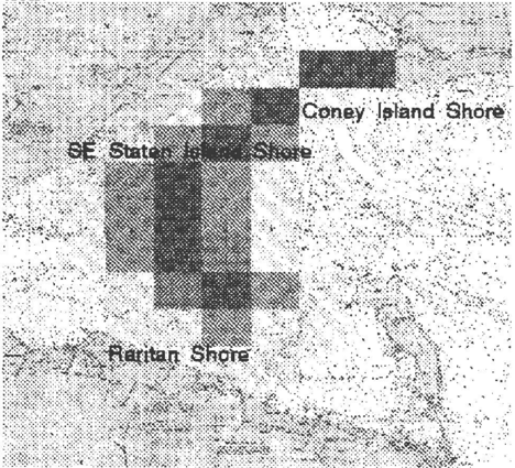
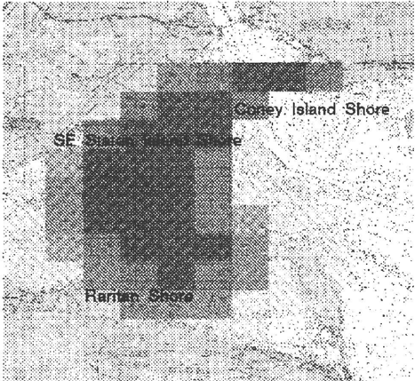
The act of surveillance to observe th e t r a j ec t o r y c ha n g e s the state of knowledge of the traje c t ory at the subsequent decision point. At this point, there will be full knowledge of the location of the oil slick. This has the side effect afforcing a re c o m p ut a t i o n using MJ, for p e r i o ds 1 to j, the transition matrices for a s p r e a d i ng rate that does not include the increase in uncertainty of the oil location over time. ( The prime signifies ob servation.) For purposes of implementation, MJ is also pre-calculated. The trajectory of qu a nt i ti e s s0·5, of the median value when the oil position is uncertain is s h o w n in Figure 1. The tra j e c t or y of actual o i l p os i tion, s is shown in Figure 2.
3.4 Representation of the Spill and Response Goals in SIPE-2
SIPE-2 plans against the forecast of the tra j e ct o r y . It has knowledge of:
- The spill rate and duration of the spill;
- The location and probability of appearance of the oil, by geographic sector, s;
- The extent {enclosing diameter) of the slick within a sector;
- The thickness of the oil slick by sector, which af fects the efficiency of oil removal.
SIPE-2 generates many possible plans of equipment employments to meet goals that derive from the de scription that it has of the trajectory. Each posted cleanup goal has a numeric value associated with it to suggest capacity of the equipment required. For ex ample, to clean up a harbor, one may need enough length of floating boom to span the harbor entrance. When running the planning system interactively, the user takes these numeric levels as suggestions of ade quate levels of response, around which the user is free to apply more equipment, or to neglect an employment goal entirely. In the combined architecture, the value of these quantities among the possible plans is deter mined by the influence diagram optimization step.
3.5 Model Simplifications Based on the Plan Output
Using SIPE-2 to construct the decision backbone from the generated plan applies the following constraints that lead to reformulations of the influence diagram and simplify its computation.
- The arrival times determined by the planner com pletely order the employment actions, reducing a par tial ordering of 2n combinations of n possible pieces equipment allocated to each location in each period, to a complete ordering.
- It is always better for equipment to arrive in a sector sooner rather than later, so the dominant choice of boom for each sector is used to restrict the boom choice for each sector. If the minimum arrival times are such that no boom would arrive in time to have any material effect on one of the threatened sensitive areas, then no action to protect it will be taken.
- The "friction" in moving equipment from one sec tor to another greatly reduces the opportunities for sequential action. The typical plan finds few reasons to move equipment once it has been deployed. Reuse takes time, and there are only two cases in the plan where it is feasible:
a)The "Observe or Disperse" decision. The choice is over which operation to perform first; to employ the one available aircraft for spreading chemical disper sants, or for surveillance on the course of the spill. The preparation and refueling times are so long that the decision reduces to either one of the other.
b )The "Chasing the spill" decision. As the spill pro gresses from the ship to the shore, should equipment
already employed somewhere else be moved in antici pation of its landfall?
Applying these constraints reduces the influence dia gram model to two periods, where the later period has options for either disperse or observe the extent of the spill, and, subsequent to the observation, for relocating equipment. The complexity of the decision sequence has been reduced to the order of 2(2n).
The codification of the USCG 's best practices as rep resented in SIPE-2 plan operators add further con straints to the optimization:
- Since booms leak, more boom is always better, but less than one times coverage of an area is useless (the oil will not be contained but just flow around), and three times coverage is the most practical. This further constrains the allocation of booms to sectors, since only boom lengths with integral converages are significant. This constrains the decision variable to a discrete value from the set {0, 1, 2, 3}, of the number of times of coverage of the area by boom. This sets the level of abstraction at which boom operations in the planner will be conveyed to the optimization com putation. (It is possible that further planning to refine individual boom operations may be done in the plan ner after number of times coverage for each sector has been optimized.)
- The earlier oil can be contained the better, since it spreads quickly.
These are the fundamental properties of the strategy that can be represented in the plan operators, wit h out recourse to detailed properties of the physical and value models. They result in further reductions in the range of choices made available in the plan output to the influence diagram.
3.6 Solution results
Further simplifications occur in computational com plexity due to the nature of the objective function.
- An ounce of costs incurred in deploying equipment clearly outweighs the pounds of cleanup costs for dam ages, should the oil reach the shore. This eliminates the need to consider deployment cost consequences of the plan actions.
- Of the boom c o m b i n a t i o n s of the 4 booms available at the three locations to be protected, all but 3 are not dominated.
These three options for boom employment are:
- equal: One layer of boom containment at the ship and at each sensitive area
- stabilize: 3 layers of boom containment around the ship, at the sacrifice of the smaller sensitive area.
- (chase to) protect: 3layers of boom to protect the smaller sensitive area, leaving the ship's leakage
uncontained.
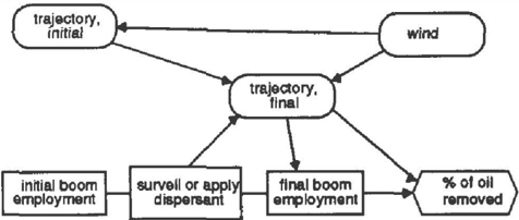
The last option must be split into two in the last pe riod, since switching to "chase to" in the second period creates a delay in arrival time of the boom and thus makes it depend on the first period choice. At this point the structure of the influence diagram and the alternatives available at each decision are defined. The diagram is shown in Figure 3.
Three options in the first and four in the second period, together with the aircraft utilization choice leave 3 x 2 x 4 = 24 plans to be evaluated by the influence diagram.
These can be further narrowed, by use of Bellman's recursion equation to solve the problem sequentially. The second period return function is
where a is aircraft employment choice, and b 2 is the second boom employment choice. V2 can be easily calculated:
| 2nd period action | aircraft | |
|---|---|---|
| surveil | disperse | |
| boom | ||
| equal | 0.29 | 0.19 |
| stablize | 0.60 | 0.17 |
| pr o t e c t | 0.17 | 0.15 |
| chase | 0.46 | 0.22 |
| (none) | 1.00 | 0.47 |
From the return function we have determined the best second period choices. There are two that are roughly tied, to either stablize or protect, while applying dis persants is always preferred. Strictly, the return func-
tion should be calculated for all values of St', and the values of St' for each first period choice substituted into the return function. That would reduce the number of plan stages we need to evaluate to 8 + 3 = 11. To verify this, Table 2 shows the computation of the final return ( the objective function over all periods) for dif ferent combinations of first and second period choices. This shows that the choices determined for the second period remain valid when all periods are considered.
| 1st period action | |||
|---|---|---|---|
| 2nd period action | equal | stablize | chase |
| equal | 0.12 | 0.11 | * |
| stabilize | 0.05 | 0.03 | * |
| protect / chase | 0.10 | 0.03 | 0.10 |
The two starred options, involve moving boom against the direction of the oil spreading ( i.e. protect in the first period, and switch in the second) and would not be considered on basic physical grounds. This could also be included as a constraint during plan generation.
The final result is that stabilize in the first period, followed by either stabilzze or chase in the second re sult in less than 3% of the oil reaching the shore that would have reached it had no controls been applied. The value of reducing uncertainty in the knowledge of the trajectory location by surveillance is minimal, and does not balance the reduction due to spreading of dis persants from the air. This says something about the "value of maneuver", to use the military metaphor, more than about the level of uncertainty in the oil trajectory. In essence, the spread of the oil is so wide that it will most likely reach all shores, and the limited ability to maneuver boom selectively to one or another turns out not to be important.
4 Conclusion
This paper has demonstrated an extreme example of how the daunting complexity of a real world domain can be made tractable by optimizing within the con straints of a combined generative planning and influ ence diagram architecture. The agent is rational only with respect to the computational limitations of the ar chitecture, hence this result is an example of bounded optimality. Had a different architecture been applied, a different result might obtain.
The argument of the paper has been that the so phisticated design of the agent can take advantage of specifics of the problem domain to simplify the compu tation. The result is a more complicated architecture, but a simpler computation; in fact, in this example, one that approaches what can be done on a spread sheet. The simplifications made within the constraints of the architecture are inspired by the characteristics of the domain. Finding them is gives a powerful tool: Perhaps not surprisingly, the richer description of the domain present in the combined architecture provides a better set of wedges that can be driven to split off large parts of the computation. The method applied is similar to "value of information" arguments; that, by knowing the available actions, their valuations and the states of knowledge under which they are taken, the constraints of the architecture do not significantly limit performance. In other terms, in cases with lim ited the flexibility, and limited range of options, the computational demands can be limited, even as the complexity and uncertainty faced may increase.
The missing link, and the task for further work is to show how the constraints that simplified the computa tional problem can be applied generally and automat ically by the generative planner on the design of the influence diagram.
Acknowledgment: This work was partially supported under U.S.DOT grants DTRS-57-G-00084 and DTRS57 -94-G-00081.
5 References
Agosta, J. M. 1995. "Formulation and implementation of an equipment configuration problem with the SIPE2 generative planner" In Proceedings of the AAAI-95 spring symposium on integrated planning applications Stanford, CA. Ma r c h 1995.
Bertsekas, D.P. 1987. Dynamic Programming: Deter ministzc and Stochastic Models, Englewood Cliffs, NJ: Prentice Hall.
Blythe, J. 1 9 9 6 . "Event-Based Decompositions for Reasoning about External Change in Planners," To appear in The Third International Conference on AI Planning Systems, Edinburgh, May 1996.
Dean, T. and M. Wellman, 1991. Planning and Con trol San Mateo, CA: Morgan Kaufmann.
Desimone, R. V. and M. desJardins. 1993. "Repre senting and Reasoning About Uncertainty during Bat tle Planning" SRI Report, number ITAD-1549-FR-93330.
Desimone, R.V. and J. M. Agosta. 1994. "Oil Spill Response Simulation: The Application of AI Planning Technology," Proceedings of the 1994 Simulation Mul ti Conference, Simulation for Emergency Management track, La Jolla, CA, April 1994.
Draper, D., S. Hanks and D. Weld. 1994. "A Proba bilistic Model of Action for Least-Commitment Plan ning with Information Gathering" In Proceedings of the Tenth Conference on Uncertainty in Artificial In telligence, Seattle, August 1994.
Goldszmidt M. and A. Darwiche. 1994. "Action Net works: A Framework for Reasoning about Actions and Change under Uncertainty" In ARPA/Rome Lab oratory Knowledge-based Planning and Scheduling Ini tiative Workshop Proceedings, Tucson, AZ, February, 1994.
Haddawy, P., A. Doan, R. Goodwin. 1995. "Efficient Decision-Theoretic Planning: Techniques and Empir ical Analysis," In Proceedings of the Eleventh Con ference on Uncertainty In Artificial Intelligence Mon treal, Canada, August 1995.
Lehner, P., C. Elaesser and S. Musman. 1994. "Con structing Belief Networks to Evaluate Plans," In AAAI Spring Symposium on Decision-Theoretic Planning, Menlo Park, CA: AAAI Press.
Lowrance, J. D. and D. E. Wilkins, 1990. "Plan evalu ation under uncertainty," in Proceedings of the Work shop on Innovative Approaches to Planning, Schedul ing and Control (K. P. Sycara, ed.), pp. 439-449, Morgan Kaufmann Publishers Inc., San Francisco, CA, Nov. 1990.
Russell, S. 1995. "Rationality and Intelligence," IJ CAI- 95, Montreal, August 1995.
Spaulding, M. 1988. "A State of the Art Review of Oil Spill Trajectory and Fate Modeling," Oil and Chem�cal Pollution, Vol. 4, pp. 39-55.
Wilkins, D. E. , K. L. Myers, J. D. Lowrance, and L. P. Wesley, 1995. "Planning and reacting in uncertain and dynamic environments," Journal of Experimental and Theoretical AI, vol. 7, no. 1, pp. 197-227,
Wilkins, D. E. 1988. Practical Planning: Extending the Classical AI Planning Parad1gm, Morgan Kauf mann Publishers Inc., San Francisco, CA