Context-Specific Independence in Bayesian Networks

Craig Boutilier

Dept. of Computer Science University of British Columbia Vancouver, BC V6T 1Z4 [email protected]

Nir Friedman

Dept. of Computer Science Stanford University Stanford, CA 94305-9010 [email protected]

Abstract

Bayesian networks provide a language for qualitatively representing the conditional independence properties of a distribution. This allows a natural and compact representation of the distribution, eases knowledge ac­ quisition, and supports effective inference algorithms. It is well-known, however, that there are certain inde­ pendencies that we cannot capture qualitatively within the Bayesian network structure: independencies that hold only in certain contexts, i.e., given a specific as­ signment of values to certain variables.. In this pa­ per, we propose a formal notion of context-specific in­ dependence (CSI), based on regularities in the condi­ tional probability tables (CPTs) at a node. We present a technique, analogous to (and based on) d-separation, for determining when such independence holds in a given network. We then focus on a particular quali­ tative representation scheme-tree-structured CPTs­ for capturing CSI. We suggest ways in which this rep­ resentation can be used to support effective inference algorithms. In particular, we present a structural de­ composition of the resulting network which can im­ prove the performance of clustering algorithms, and an alternative algorithm based on cutset conditioning.

1 Introduction

The power of Bayesian Network (BN) representations of probability distributions lies in the efficient encoding of in­ dependence relations among random variables. These in­ dependencies ares;_� to provide savings in the rep­ resentation of a distribution, ease of knowledge acquisition and domain modeling, and computational savings in the in­ ference process.1 The objective of this paper is to increase this power by refining the BN representation to capture ad­ ditional independence relations. In particular, we investi­ gate how independence given certain variable assignments

1 Inference refers to the computation of a posterior distribution, conditioned on evidence.

Moises Goldszmidt

SRI International 333 Ravenswood Way, EK329 Menlo Park, CA 94025 [email protected]

Daphne Koller

Dept. of Computer Science Stanford University Stanford, CA 94305-9010 [email protected] can be exploited in BNs in much the same way indepen­ dence among variables is exploited in current BN represen­ tations and inference algorithms. We formally chatacterize this structured representation and catalog a number of the advantages it provides.

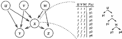
A BN is a directed acyclic graph where each node rep­ resents a random variable of interest and edges represent direct correlations between the variables. The absence of edges between variables denotes statements of indepen­ dence. More precisely, we say that variables Z andY are independent given a set of variables X if P(z I :c, y) = P(z [ x ) for all values x, y and z of variables X, Y and Z. A BN encodes the following statement of independence about each random variable: a variable is independent of its non-descendants in the network given the state of its patents [14]. For example, in the network shown in Figure I, Z is independent of U, V andY given X and W. Further inde­ pendence statements that follow from these local statements can be read from the network structure, in polynomial time, using a graph-theoretic criterion called d-separation [14].

In addition to representing statements of independence, a BN also represents a particular distribution (that satisfies all the independencies). This distribution is specified by a set of conditional probability tables (CPTs). Each node X has an associated CPT that describes the conditional distribu­ tion of X given different assignments of values for its par­ ents. Using the independencies encoded in the structure of the network, the joint distribution can be computed by sim­ ply multiplying the CPTs.

In its most naive form, a CPT is encoded using a tabular representation in Which each assignment of values to the parents of X requires the specification of a conditional dis­ tribution over X. Thus, for example, assuming that all of U, V, Wand X in Figure 1 are binary, we need to spec­ ify eight such distributions (or eight parameters). The size of this representation is exponential in the number of par­ ents. Furthermore, this representation fails to capture cer­ tain regularities in the node distribution. In the CPT of Figure 1, for example, P(x I u, V, W) is equal to some constant p1 regardless of the values taken by V and W: when u holds (i.e., when U = t) we need not consider

the values of V and W. Clearly, we need to specify at most five distributions over X instead of eight. Such reg­ ularities occur often enough that at least two well known BN products-Microsoft's Bayesian Networks Modeling Tool and Knowledge Industries' DXpress-have incorpo­ rated special mechanisms in their knowledge acquisition in­ terface that allow the user to more easi ly specify the corre­ sponding CPTs.

In this paper, we provide a formal foundation for such reg­ ularities by using the notion of context-specific indepen­ dence. Intuitively, in our example, the regularities in the CPT of X ensure that X is independent of W and V given the context u (U = t), but is dependent on W, V in the con­ text u (U = f). This is an assertion of context-specific in­ dep en de n c e (CSI), which is more r es tr ic ted than the s tat e­ ments of variable independence that are encoded by the BN structure. Nevertheless, as we show in this paper, such statements can be used to extend the advantages of variable independence for probabilistic inference, namely, ease of knowledge elicitation, compact representation and compu­ tational benefits in inference,

We are certainly not the first to suggest extensions to the BN representation in order to capture additional indepen­ dencies and (potentially) enhance inference. Well-known examples include Heckerman's [9] similarity networks (and the related multinets [7]), the use of asymmetric represen­ tations for decision making [18, 6] and Poole's [16] use of probabilistic Horn rules to encode dependencies between variables. Even the representation we emphasize (decision trees) have been used to encode CPTs [2, 8]. The intent of this work is to formalize the notion of CSI, to study its rep­ resentation as part of a more general framework, and to pro­ pose methods for utilizing these representations to enhance probabilistic inference algorithms.

We begin in Section 2 by defining context-specific indepen­ dence formally, and introducing a simple, local transforma­ tion for a BN based on arc deletion so that CSI statements can be readily determined us i n g d-separation. Section 3 dis­ cusses in detail how trees can be used to represent CPTs compactly, and how this representation can be exploited by the algorithms for determining CSI. Section 4 offers sug­ gestions for speeding up probabilistic inference by taking advantage of CSI. We present network transformations that may reduce clique size for clustering algorithms, as well as techniques that use CSI-and the associated arc-deletion s t r a teg y -i n cutset conditioning. We conclude with a dis­ cussion of related notions and future research directions.

2 Context-Specific Independence and Arc Deletion

Consider a finite set U = {X 1 , ... , X n} of discrete ran­ dom variables where each variable X; E U may take on values from a finite domain. We use capital letters, such as X, Y, Z, for variable names and lowercase letters x, y, z to denote specific values taken by those variables. The set of all values of X is denoted val ( X). Sets of variables are de­ noted by boldface capital letters X, Y, Z, and as s ig n men ts of values to the variables in these sets will be denoted by boldface lowercase letters a:, y, z (we use val ( X) in the ob­ vious way).

Definition 2.1: Let P be a joint probability distribution over the variables in U, and let X, Y, Z be subsets of U. X and Y are conditionally independent given Z, denoted I(X; Y I Z), iffor all a: E vai(X), y E v a i( Y ) , z E val(Z), the following relationship holds:

We summarize this last statement (for all values of a:, y, z) by P(X I z, Y) = P(X I Z).

A Bayesian network is a directed acyclic graph B whose nodes correspond to the random variables X 1 , ... , X n, and whose edges represent direct dependencies between the variables. The graph structure of B encodes the set of inde­ pendence assumptions representing the assertion that each node X; is independent of its non-descendants given its par­ ents Ilx 1 · These statements are local, in that they involve only a node and its parents in B. Other I() statements, in­ volving arbitrary sets of v ar i a bl e s , follow from these local assertions. These can be read from the structure of B us­ ing a graph-theoretic path criterion called d-separation [ 14] that can be tested in polynomial time.

A BN B represents independence information about a par­ ticular distribution P. Thus, we require that the indepen­ dencies encoded in B hold for P. More precisely, B is said to be an /-map for the distribution P if every independence sanctioned by d-separation in B holds in P, A BN is re­ quired to be a minimal 1-map, in the sense that the deletion of any edge in the network destroys the 1-mapness of the network with respect to the distribution it describes. A BN B for P permits a compact representation of the distribu­ tion: we need only specify, for each variable X;, a condi­ tional probability table (CPT) encoding a parameter P(x; I U,,) for each possible value of the variables in {X;, Ilx, }. (See [14] for details.)

The graphical structure of the BN can only capture indepen­ dence relations of the form I(X; Y I Z), that is, indepen­ dencies that hold for any assignment of values to the vari­ ables in Z. However, we are often interested in indepen­ dencies that hold only in certain contexts.

Definition 2.2: Let X, Y, Z, C be pairwise disjoint sets of variables. X and Y are contextually independent given

Z and the c ontexte E val( C), denoted Ic(X; Y I Z, c ) , if P(X I Z, c, Y) = P(X I Z, c ) whenever P(Y, Z, c) > 0.

This assertion is similar to that in Equation ( 1 ) , taking CUZ as evidence, but requires that the independence of X and Y hold only for the particular assignment c to C.

It is easy to see that certain local Ic statements -those of the form Ic(X; Y I c) for Y, C c;;; IIxcan be veri­ fied by direct examination of the CPT for X. In Figure 1, for example, we can verify Ic (X; V I u) by checking in the CPT for X whether, for each value w ofW, P(X I v, w, u ) does not depend on v (i.e., it is the same for all values v of V). The next section explores different representations of the CPTs that will allow us to check these local statements efficiently. Our objective now is to establish an analogue to the principle of d-separation: a computationally tractable method for deciding the validity of non-local Ic statements. It turns out that this problem can be solved by a simple re­ duction to a problem of validating variable independence statements in a simpler network. The latter problem can be efficiently solved using d-separation.

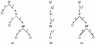
Definition 2.3: An edge from Y into X will be called v ac ­ u ous in B , given a context c, if Ic(X; Y I c n IIx ). Given BN Band a context c, we define B ( c ) as theBN that results from deleting vacuous edges in B given c. We say that X is CSI-separated from Y given Z in context c in B if X is d-separated from Y given Z U C in B (c).

Note that the statement Ic (X; y I c n IIx) is a local Ic statement and can be determined by inspecting the CPT for X. Thus, we can decide CSI-separation by transforming B into B ( c) using these local Ic statements to delete vacuous edges, and then usingd-separation on the resulting network.

We now show that this notion of CSI-separation is sound and (in a strong sense) complete given these local indepen­ dence statements. Let B be a network structure and I: be a set of local Ic statements over B. We say that ( B, z;) is a CS/-map of a distribution P if the independencies im­ pliedby(B,I�)hold inP,i.e.,Ic(X;Y I Z,c)holds in P whenever X is CS/-separated from Y given Z in con­ text c in ( B , I;). We say that (B, I;) is a peifect CSI-map if the implied independencies are the only ones that hold in P, i.e., if Ic(X; Y I Z, c ) if and onlyif X is CSJ-separated from Y given Z in context c in (B,In

Theorem 2.4: Let B be a network structure, I� be a set of local independencies, and P a distribution consistent with B and I;. Then ( B ,I;) is a CSI-mapof P.

The theorem establishes the soundness of this procedure. Is the procedure also complete? As for any such procedure, there may be independencies that we cannot detect using only local independencies and network structure. However, the following theorem shows that, in a sense, this procedure provides the best results that we can hope to derive based solely on the structural properties of the distribution.

Theorem 2.5: Let B be a network structure, I; be a set of local independencies. Then there exists a distribution P, c onsistent w ith B and I;, such that (B, I;) is a perfect CSJ­ mapof P.

3 Structured Representations of CPTs

Context-specific independence corresponds to regularities within CPTs. In this section, we discuss possible represen­ tations that capture this regularity qualitatively, in much the same way that a BN structure qualitatively captures condi­ tional independence. Such representations admit effective algorithms for determining local CSI statements and can be exploited in probabilistic inference. For reasons of space, we focus primarily on tree-structured representations.

In general, we can view a CPT as a function that maps val(ITx) into distributions over X. A compact represen­ tation of CPTs is simply a representation of this function that exploits the fact that distinct elements of val(IIx) are associated with the same distribution. Therefore, one can compactly represent CPTs by simply partitioning the space val(IIx) into regions mapping to the same distribution.

Most generally, we can represent the partitions using a set of mutually exclusive and exhaustive generalized proposi­ tions over the variable set ITx. A generalized proposition is simply a truth functional combination of specific variable assignments, so that if Y, Z E IIx, we may have a par­ tition characterized by the generalized proposition (Y = y) V -.(Z = z ) . Each such proposition is associated with a distribution over X. While this representation is fully gen­ eral, it does not easily support either probabilistic inference or inference about CSI. Fortunately, we can often use other, more convenient, representations for this type of partition­ ing. For example, one could use a canonical logical form such as minimal CNF. Classification trees (also known in the machine learning community as decision trees) are an­ other popular function representation, with partitions of the state space induced by the labeling of branches in the tree. These representations have a number of advantages, includ­ ing the fact that vacuous edges can be detected, and reduced CPTs produced in linear time (in the size of the CPT repre­ sentation). As expected, there is a tradeoff: the most com­ pact CNF or tree representation of a CPT might be much larger (exponentially larger in the worst case) than the min­ imal representation in terms of generalized propositions.

For the purposes of this paper, we focus on CPT-trees­ tree-structured CPTs, deferring discussion of analogous re­ sults for CNF representations and graph-structured CPTs (of the form discussed by [3]) to a longer version of this paper. A major advantage of tree structures is their nat­ uralness, with branch labels corresponding in some sense to "rule" structure (see Figure I). This intuition makes it particularly easy to elicit probabilities directly from a hu­ man expert. As we show in subsequent sections, the tree structure can also be utilized to speed up BN inference al­ gorithms. Finally, as we discuss in the conclusion, trees are also amenable to well-studied approximation and learning

methods [17]. In this section, we show that they admit fast algorithms for detecting CSI.

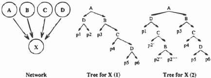
In general, there are two operations we wish to perform given a context c: the first is to determine whether a given arc into a variable X is vacuous; the second is to determine a reduced CPT when we condition on c. This operation is carried out whenever we set evidence and should reflect the changes to X's parents that are implied by context-specific independencies given c. We examine how to perform both types of operations on CPT-trees. To avoid confusion, we use t-node and t-are to denote nodes and arcs in the tree (as opposed to nodes and arcs in the BN). To illustrate these ideas, consider the CPT-tree for the variable X in Figure 2. (Left t-ares are labeled true and right t-ares false).

Given this representation, it is relatively easy to tell which parents are rendered independent of X given context c. As­ sume that Tree l represents the CPT for X. In context a, clearly D remains relevant while C and B are rendered in­ dependent of X. Given a 1\ b, both C and D are rendered independent of X. Intuitively, this is so because the distri­ bution on X does not depend on C and D once we know c = a 1\ b: every path from the root to leaf which is consis­ tent with c fails to mention Cor D.

Definition 3.1: A path in the CPT-tree is the set of t-ares lying between the root and a leaf. The labeling of a path is the assignment to variables induced by the labels on the t­ ares of the path. A variable Y occurs on a path if one of the t-nodes along the path tests the value ofY. A path is consis­ tent with a context c iff the labeling of the path is consistent with the assignment of values in c.

Theorem 3.2: Let T be a CPT-tree for X and let Y be one of its parents. Let c E C be some context (Y (/:. C). If Y does not lie on any path consistent with c, then the edge Y -+ X is vacuous given c.

This provides us with a sound test for context-specific in­ dependence (only valid independencies are discovered). However, the test is not complete, since there are CPT struc­ tures that cannot be represented minimally by a tree. For in­ stance, suppose that pl = p5 and p2 = p6 in the example above. Given context bAc, we can tell that A is irrelevant by inspection; but, the choice of variable ordering prevents us from detecting this using the criterion in the theorem. How­ ever, the test above is complete in the sense that no other edge is vacuous given the tree structure.

Theorem 3.3: LetT be a CPT-tree for X, letY E Ilx and let c E C be some context (Y (/:. C). IfY occurs on a path that is consistent with c, then there exists an assignment of parameters to the leaves ofT such that Y -+ X is not vac­ uous given c.

This shows that the test described above is, in fact, the best test that uses only the structure of the tree and not the ac­ tual probabilities. This is similar in spirit to d-separation: it detects all conditional independencies possible from the structure of the network, but it cannot detect independen­ cies that are hidden in the quantification of the links. As for conditional independence in belief networks, we need only soundness in order to exploit CSI in inference.

It is also straightforward to produce a reduced CPT-tree rep­ resenting the CPT conditioned on context c. Assume c an assignment to variables containing certain parents of X and T is the CPT-tree of X, with root R and immediate sub­ trees T1, · · ·Tk. The reduced CPT-tree T(c) is defined re­ cursively as follows: if the label of R is not among the vari­ ables C, then T(c) consists of R with subtrees Tj (c); if the labelofRis someY E C,thenT(c) = 7j(c),whereTj is the subtree pointed to by the t-are labeled with value y E c. Thus, the reduced tree T(c) can be produced with one tree traversal in O(ITI) time.

Proposition 3.4: Variable Y labels some t-node in T(c) if and only if Y ¢ C and Y occurs on a path in T that is consistent with c.

This implies that Y appears in T( c) if and only if Y -+ X is not deemed vacuous by the test described above. Given the reduced tree, determining the list of arcs pointing into X that can be deleted requires a simple tree traversal ofT( c ) . Thus, reducing the tree gives us an efficient and sound test for determining the context-specific independence of all parents of X.

4 Exploiting CSI in Probabilistic Inference

Network representations of distributions offer considerable computational advantages in probabilistic inference. The graphical structure of a BN lays bare variable independence relationships that are exploited by well-known algorithms when deciding what information is relevant to (say) a given query, and how best that information can be summarized. In a similar fashion, compact representations of CPTs such as trees make CSI relationships explicit. In this section, we de­ scribe how CSI might be exploited in various BN inference algorithms, specifically stressing particular uses in cluster­ ing and cutset conditioning. Space precludes a detailed pre­ sentation; we provide only the basic intuitions here. We also emphasize that these are by no means the only ways in which BN inference can employ CSI.

4.1 Network Transformations and Clustering

The use of compact representations for CPTs is not a novel idea. For instance, noisy-or distributions (or generaliza­ tions [19]) allow compact representation by assuming that the parents of X make independent "casual contributions" to the value of X. These distributions fall into the gen­ eral category of distributions satisfying causal indepen­ dence [10, 11). For such distributions, we can perform a structural transformation on our original network, resulting in a new network where many of these independencies are encoded qualitatively within the network structure. Essen­ tially, the transformation introduces auxiliary variables into the network, then connects them via a cascading sequence of deterministic or-nodes [11). While CSI is quite distinct from causal independence, similar ideas can be applied: a structural network transformation can be used to capture certain aspects of CSI directly within the EN-structure.

Such transformations can be very useful when one uses an inference algorithm based on clustering [13]. Roughly speaking, clustering algorithms construct a join tree, whose nodes denote (overlapping) clusters of variables in the orig­ inal BN. Each cluster, or clique, encodes the marginal dis­ tribution over the set val(X) of the nodes X in the cluster. The inference process is carried out on the join tree, and its complexity is determined largely by the size of the largest clique. This is where the structural transformations prove worthwhile. The clustering process requires that each fam­ ily in the BN- a node and its parents- be a subset of at least one clique in the join tree. Therefore, a family with a large set of values val ( { X; } U ITx,) will lead to a large clique and thereby to poor performance of clustering algo­ rithms. A transformation that reduces the overall number of values present in a family can offer considerable computa­ tional savings in clustering algorithms.

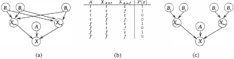
In order to understand our transformation, we first consider a generic node X in a Bayesian network. Let A be one of X's parents, and let B1, ... , Bk be the remaining par­ ents. Assume, for simplicity, that X and A are both binary­ valued. Intuitively, we can view the value of the random variable X as the outcome of two conditional variables: the value that X would take if A were true, and the value that X would take if A were false. We can conduct a thought ex­ periment where these two variables are decided separately, and then, when the value of A is revealed, the appropriate value for X is chosen.

Formally, we define a random variable X A=t, with a condi­ tional distribution that depends only on B 1, . .. , Bk:

We can similarly define a variable XA=f. The variable X is equal to X A=t if A = t and is equal to XA= f if A = f. Note that the variables XA=t and XA=J both have the same set of values as X . This perspective allows us to replace the node X in any network with the subnetwork illustrated in Figure 3(a). The node X is a deterministic node, which we call a multiplexer node (since X takes either the value of XA=t or of X A-:= f , depending on the value of A). Its CPT is presented in Figure 3(b).

For a generic node X, this decomposition is not particularly useful. For one thing, the total size of the two new CPTs is exactly the same as the size of the original CPT for X; for another, the resulting structure (with its many tightly­ coupled cycles) does not admit a more effective decompo­ sitions into cliques. However, if X exhibits a significant amount of CSI, this type of transformation can result in a far more compact representation. For example, let k = 4, and assume that X depends only on B1 and B2 when A is true, and only on B3 and B4 when A is false. Then each of X A=t and XA=f will have only two parents, as in Figure 3(c). If these variables are binary, the new representation requires two CPTs with four entries each, plus a single determinis­ tic multiplexer node with 8 (predetermined) 'distributions'. By contrast, the original representation of X had a single CPT with 32 entries. Furthermore, the structure of the re­ sulting network may well allow the construction of a join tree with much smaller cliques.

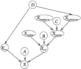
Our transformation uses the structure of a CPT-tree to ap­ ply this decomposition recursively. Essentially, each node X is first decomposed according to the parent A which is at the root of its CPT tree. Each of the conditional nodes (X A=t and XA=f in the binary case) has, as its CPT, one of the subtrees of the t-node A in the CPT for X. The result­ ing conditional nodes can be decomposed recursively, in a similar fashion. In Figure 4, for example, the node corre­ sponding to XA=J can be decomposed into XA=J,B=t and XA=f,B=J. The node XA=J,B=f can then be decomposed

into XA=J,B=J,C=t and XA=f,B=J,C=f.

The nodes XA=J,B=t and XA=J,B=J,C=t cannot be de­ composed further, since they have no parents. While further decomposition of nodes XA=t and XA=f,B=f,C=f is pos­ sible, this is not beneficial, since the CPTs for these nodes are unstructured (a complete tree of depth 1 ). It is clear that this procedure is beneficial only if there is a structure in the CPT of a node. Thus, in general, we want to stop the decomposition when the CPT of a node is a full tree. (Note that this includes leaves a special case.)

As in the structural transformation for noisy-or nodes of [11], our decomposition can allow clustering algorithms to form smaller cliques. After the transformation, we have many more nodes in the network (on the order of the size of all CPT tree representations), but each generally has far fewer parents. For example, Figure 4 describes the transfor­ mation of the CPT of Tree (1) of Figure 2. In this transfor­ mation we have eliminated a family with four parents and introduced several smaller families. We are currently work­ ing on implementing these ideas, and testing their effective­ ness in practice. We also note that a large fraction of the auxiliary nodes we introduce are multiplexer nodes, which are deterministic function of their parents. Such nodes can be further exploited in the clustering algorithm [12].

We note that the reduction in clique size (and the result­ ing computational savings) depend heavily on the structure of the decision trees. A similar phenomenon occurs in the transformation of [11], where the effectiveness depends on the order in which we choose to cascade the different par­ ents of the node.

As in the case of noisy-or, the graphical structure of our (transformed) BN cannot capture all independencies im­ plicit in the CPTs. In particular, none of the CSI relations­ induced by particular value assignments-can be read from the transformed structure. In the noisy-or case, the analogue is our inability to structurally represent that a node's parents are independent if the node is observed to be false, but not if it is observed to be true. 2 In both cases, these CSI rela­ tions are captured by the deterministic relationships used in the transformation: in an "or" node, the parents are inde­ pendent if the node is set to false. In a multiplexer node, the value depends only on one parent once the value of the "selectin.;" parent (the original variable) is known.

4.2 Cutset Conditioning

Even using noisy-or or tree representations, the join-tree al­ gorithm can only take advantage of fixed structural inde­ pendencies. The use of s ta t ic precompilation makes it diffi­ cult for the algorithm to take advantage of independencies that only occur in certain circumstances, e.g., as new ev­ idence arrives. More dynamic algorithms, such as cutset conditioning [14], can exploit context-specific independen­ cies more effectively. We investigate below how cutset al­ gorithms can be modified to exploit CSI using our decision­ tree representation. 3

The cutset conditioning algorithm works roughly as fol­ lows. We select a cutset, i.e., a set of variables that, once in­ stantiated, render the network singly connected. Inference is then carried out using reasoning by cases, where each case is a possible assignment to the variables in the cutset C. Each such assignment is instantiated as evidence in a call to the polytree algorithm [14], which performs infer­ ence on the resulting network. The results of these calls are combined to give the final answer. The running time is largely determined by the number of calls to the poly tree al­ gorithm (i.e., Ivai( C) I).

CSI offers a rather obvious advantage to inference algo­ rithms based on the conditioning of loop cutsets. By in­ stantiating a particular variable to a certain value in order to cut a loop, CSI may render other arcs vacuous, perhaps cut­ ting additional loops without the need for instantiating addi­ tional variables. For instance, suppose the network in Fig­ ure 1 is to be solved using the cutset { U, V, W} (this might be the optimal strategy if I val ( X) I is very large). Typically, we solve the reduced singly-connected network lval(U)I · lval(V) l·lval(W) I times, once for each assignment of val­ ues to U, V, W. However, by recognizing the fact that the connections between X and {V, W} are vacuous in context u, we need not instantiate V and W when we assign U = t. This replaces Jval(V) I · I val( W) I network evaluations with a single evaluation. However, when U = f, the instanti­ ation of V, W can no longer be ignored (the edges are not vacuous in context u).

To capture this phenomenon, we generalize the standard no­ tion of a cutset by considering tree representations of cut­ sets. These reflect the need to instantiate certain variables in some contexts, but not in others, in order to render the net­ work singly-connected. Intuitively, a conditional cutset is a tree with interior nodes labeled by variables and edges Ia-

z This last fact is heavily utilized by algorithms targeted specif­ ically at noisy-or networks (mostly BN20 networks).

3 We believe similar ideas can be applied to other compact CPT representations such as noisy-or.

beled by (sets of) variable values.4 Each branch through the tree corresponds to the set of assignments induced by fixing one variable value on each edge. The tree is a conditional cutset if: (a) each branch through the tree represents a con­ text that renders the network singly-connected; and (b) the set of such assignments is mutually exclusive and exhaus­ tive. Examples of conditional cutsets for the BN in Figure 1 are illustrated in Figure 5: (a) is the obviouscompact cutset; (b) is the tree representation of the "standard" cutset, which fails to exploit the structure of the CPT, requiring one eval­ uation for each instantiation of U, V, W.

Once we have a conditional cutset in hand, the extension of classical cutset inference is fairly obvious. We con­ sider each assignment of values to variables determined by branches through the tree, instantiate the network with this assignment, run the poly tree algorithm on the resulting net­ work, and combine the results as usual.5 Clearly, the com­ plexity of this algorithm is a function of the number of dis­ tinct paths through the conditional cutset. It is therefore cru­ cial to find good heuristic algorithms for constructing small conditional cutsets. We focus on a "computationally inten­ sive" heuristic approach that exploits CSI and the existence of vacuous arcs maximally. This algorithm constructs con­ ditional cutsets incrementally, in a fashion similar to stan­ dard heuristic approaches to the problem [20, 1]. We dis­ cuss computationally-motivated shortcuts near the end of this section.

The standard "greedy" approach to cutset construction selects nodes for the cutset according to the heuristic value �fi?, where the weight w(X) of variable X is log(lval(X)I) and d(X) is the out-degree of X in the net­ work graph [20, 1]. 6 The weight measures the work needed to instantiate X in a cutset, while the degree of a vertex gives an idea of its arc-cutting potential-more incident outgoing edges mean a larger chance to cut loops. In order to extend this heuristic to deal with CSI, we must estimate the extent to which arcs are cut due to CSI. The obvious approach, namely adding to d(X) the number of arcs actu­ ally rendered vacuous by X (averaging over values of X), is reasonably straightforward, but unfortunately is somewhat

4 We explain the need for set-valued arc labels below.

5 As in the s tan dard c uts e t a l g orit h m , the weights required to combine the answers from the d iff e r e n t cases can be obtained from the polytr ee co mp u t a t i ons [21].

6 We assume that the network has been preprocessed by node­ splitting so that legitimate cutsets can be selected e as i ly . See [ 1] for details.

myopic. In particular, it ignores the potential for arcs to be cut subsequently. For example, consider the family in Fig­ ure 2, with Tree 2 reflecting the CPT for X. Adding A or B to a cutset causes no additional arcs into X to be cut, so they will have the same heuristic value (other things being equal). However, clearly A is the more desirable choice be­ cause, given either value of A, the conditional cutsets pro­ duced subsequently using B, C and D will be very small.

Rather than using the actual n u m b e r of arcs cut by s ele c t ­ ing a node for the cutset, we should consider the expected number of arcs that will be cut. We do this by consider­ ing, for each of the children V of X, how many distinct probability entries (distributions) are found in the structured representation of the CPT for that child for each instantia­ tion X = x; (i.e., the size of the reduced CPT). The log of this value is the expected number of parents required for the child V after X = Xi is known, with fewer parents indicating more potential for arc-cutting. We can then av­ erage this number for each of the values X may take, and sum the expected number of cut arcs for each of X's chil­ dren. This measure then plays the role of d(X) in the cutset heuristic. More precisely, let t(V) be the size of the CPT­ structure (i.e., number of entries) for V in a fixed network; and let t(V, xi ) be the size of the reduced CPT given con­ text X = xi (we assume X is a parent of V). We define the expected number of parents of V given xi to be

The expected number of arc deletions from B if X is instan­ tiated is given by

Thus, ;,��� gives an reasonably accurate picture of the value of adding X to a conditional cutset in a network B.

Our cutset construction algorithm proceeds recursively by: 1) adding a heuristically selected node X to a branch of the tree-structured cutset; 2) adding t-ares to the cutset-tree for each value x; E val(X); 3) constructing a new network for each of these instantiations of X that reflects CSI; and 4) extending each of these new arcs recursively by selecting the node that looks best in the new network corresponding to that branch. We can very roughly sketch it as follows. The algorithm begins with the original network B.

1. Remove singly-connected nodes from B, leaving Br. If no nodes remain, return the empty cutset-tree.
2. Choose node X in Br s.t. w(X)Jd'(X) is minimal.

3. For each x; E val(X), construct Bx, by removing vacuous arcs from Br and replacing all CPTs by the reduced CPTs using X = x;.

4. Return the tree T' where: a) X labels the root ofT'; b) one t-are for each x; emanates from the root; and c)

the t-node attached to the end of the x; t-are is the tree produced by recursively calling the algorithm with the network B:x, .

Step 1 of the algorithm is standard [20, 1 ]. In Step 2, it is im­ portant to realize that the heuristic value of X is determined with respect to the current network and the context already established in the existing branch of the cutset. Step 3 is required to ensure that the selection of the next variable re­ flects the fact that X = Xi is part of the current context. Fi­ nally, Step 4 emphasizes the conditional nature of variable selection: different variables may be selected next given different values of X. Steps 2-4 capture the key features of our approach and have certain computational implications, to which we now turn our attention.

Our algorithm exploits CSI to a great degree, but requires computational effort greater than that for normal cutset con­ struction. First, the cutset itself is structured: a tree rep­ resentation of a standard cutset is potentially exponentially larger (a full tree). However, the algorithm can be run on­ line, and the tree never completely stored: as variables are instantiated to particular values for conditioning, the selec­ tion of the next variable can be made. Conceptually, this amounts to a depth-first construction of the tree, with only one (partial or complete) branch ever being stored. In ad­ dition, we can add an optional step before Step 4 that de­ tects structural equivalence in the networks Bx, . If, say, the instantiations of X to x; and xi have the same structural effect on the arcs in B and the representation of reduced CPTs, then we need not distinguish these instantiations sub­ sequently (in cutset construction). Rather, in Step 4, we would create one new t-are in the cutset-tree labeled with the set {xi , Xj } (as in Figure 5). This reduces the number of graphs that need to be constructed (and concomitant com­ putations discussed below). In completely unstructured set­ tings, the representation of a conditional cutset would be of size similar to a normal cutset, as in Figure 5(b).

Apart from the amount of information in a conditional cut­ set, more effort is needed to decide which variables to add to a branch, since the heuristic component d' (X) is more in­ volved than vertex degree. Unfortunately, the value d'(X) is not fixed (in which case it would involve a single set of prior computations); it must be recomputed in Step 2 to re­ flect the variable instantiations that gave rise to the current network. Part of the re-evaluation of d'(X) requires that CPTs also be updated (Step 3). Fortunately, the number of CPTs that have to be updated for assignment X = x; is small: only the children of X (in the current graph) need to have CPTs updated. This can be done using the CPT reduction algorithms described above, which are very effi­ cient. These updates then affect the heuristic estimates of only their parents; i.e., only the "spouses" V of X need to have their value d'(V) recomputed. Thus, the amount of work required is not too large, so that the reduction in the number of network evaluations will usually compensate for the extra work. We are currently in the process of imple­ menting this algorithm to test its performance in practice.

There are several other directions that we are currently in­ vestigating in order to enhance this algorithm. One involves developing less ideal but more tractable methods of con­ ditional cutset construction. For example, we might select a cutset by standard means, and use the considerations de­ scribed above to order (on-line) the variable instantiations within this cutset. Another direction involves integrating these ideas with the computation-saving ideas of [4] for standard cutset algorithms.

5 Concluding Remarks

We have defined the notion of context-specific indepen­ dence as a way of capturing the independencies induced by specific variable assignments, adding to the regularities in distributions representable in BNs. Our results provide foundations for CSI, its representation and its role in infer­ ence. In particular, we have shown how CSI can be deter­ mined using local computation in a BN and how specific mechanisms (in particular, trees) allow compact representa­ tion of CPTs and enable efficient detection of CSI. Further­ more, CSI and tree-structured CPT s can be used to speed up probabilistic inference in both clustering and cutset-style al­ gorithms.

As we mentioned in the introduction, there has been con­ siderable work on extending the BN representation to cap­ ture additional independencies. Our notion of CSI is re­ lated to what Heckerman calls subset independence in his work on similarity networks [9] . Yet, our approach is sig­ nificantly different in that we try to capture the additional independencies by providing a structured representation of the CPTs within a single network, while similarity networks and multinets [9, 7] rely on a family of networks. In fact the approach we described based on decision trees is closer in spirit to that of Poole's rule-based representations of net­ works [ 1 6] .

The arc-cutting technique and network transformation in­ troduced in Section 2 is reminiscent of the network trans­ formations introduced by Pearl in his probabilistic calculus of action [ 1 5] . Indeed the semantics of actions proposed in that paper can be viewed as an instance of CSI. This is not a mere coincidence, as it is easy to see that networks representing plans and influence diagrams usually contain a significant amount of CSI. The effects of actions (or de­ cisions) usually only take place for specific instantiation of some variables, and are vacuous or trivial when these in­ stantiations are not realized. Testimony to this fact is the work on adding additional structure to influence diagrams by Smith et al. [ 1 8], Fung and Shachter [6], and the work by Boutilier et al [2] on using decision trees to represent CPTs in the context of Markov Decision Processes.

There are a number of future research directions that are needed to elaborate the ideas presented here, and to expand the role that CSI and compact CPT representations play in probabilistic reasoning. We are currently exploring the use of different CPT representations, such as decision graphs, and the potential interaction between CSI and causal inde-

pendence (as in the noisy-or model). A deeper examina­ tion of the network transformation algorithm of Section 4. 1 and empirical experiments are necessary to determine the circumstances under which the reductions in clique size are significant. Similar studies are being conducted for the con­ ditional cutset algorithm of Section 4.2 (and its variants). In particular, to determine the extent of the overhead involved in conditional cutset construction. We are currently pursu­ ing both of these directions.

CSI can also play a significant role in approximate prob­ abilistic inference. In many cases, we may wish to trade a certain amount of accuracy to speed up inference, allow more compact representation or ease knowledge acquisi­ tion. For instance, a CPT exhibiting little structure (i.e., little or no CSI) cannot be compactly represented; e.g., it may require a full tree. However, in many cases, the local dependence is weaker in some circumstances than in oth­ ers. Consider Tree 2 in Figure 2 and suppose that none of p2', p2" , p2'" are very different, reflecting the fact the influ­ ence of B and C's on X is relatively weak in the case where A is true and D i s false. In this case, we may assume that these three entries are actually the same, thus approximat­ ing the true CPT using a decision tree with the structure of Tree 1.

This saving (both in representation and inference, using the techniques of this paper) comes at the expense of accu­ racy. In ongoing work, we show how to estimate the (cross­ entropy) error of a local approximation of the CPTs, thereby allowing for practical greedy algorithms that trade off the error and the computational gain derived from the simpli­ fication of the network. Tree representations turn out to be particularly suitable in t h i s regard. In particular, we show that decision-tree construction algorithms from the machine learning community can be used to construct an appropriate CPT-tree from a full conditional probability table; pruning algorithms [ 1 7] can then be used on this tree, or on one ac­ quired directly from the user, to simplify the CPT -tree in or­ der to allow for faster inference.

Structured representation of CPTs have also proven benefi­ cial in learning Bayesian networks from data [ 5]. Due to the compactness of the representation, learning procedures are capable of inducing networks that better emulate the true complexity of the interactions present in the data.

This paper represents a starting point for a rigorous ex­ tension of Bayesian network representations to incorporate context-specific independence. As we have seen, CSI has a deep and far-ranging impact on the theory and practice of many aspects of probabilistic inference, including rep­ resentation, inference algorithms, approximation and learn­ ing. We consider the exploration and development of these ideas to be a promising avenue for future research.

Acknowledgements: We would like to thank Dan Geiger, Adam Grove, Daishi Harada, and Zohar Yakhini for useful discussions. Some of this work was performed while Nir Friedman and Moises Goldszmidt were at Rockwell Palo Alto Science Center, and Daphne Koller was at U.C. Berke- ley. This work was supported by a University of California President's Postdoctoral Fellowship (Koller), ARPA con­ tract F30602-95-C-0251 (Goldszmidt), an IBM Graduate fellowship and NSF Grant IRI-95-03109 (Friedman), and NSERC Research Grant OGP0121 843 (Boutilier).

References

• [ 1 ] A. Becker and D. Geiger. Approximation algorithms for the loop cutset problem. In UAJ-94, pp. 60-68, 1994.
• C. Boutilier, R. Dearden, and M. Goldszmidt. Exploiting structure in policy construction. In /JCA/-95, pp. 1 1 04-1 1 1 1 , 1995.
• R. E. Bryant. Graph-based algorithms for boolean func­ tion manipulation. IEEE T ransactions on Computers, C35(8):677-691 ' 1986.
• A. Darwiche. Conditioning algorithms for exact and approx­ imate inference in causal networks. In UAI-95, pp. 99-107, 1995.
• N. Friedman and M. Goldszmidt. Learning Bayesian net­ works with local structure. In UAI '96, 1 996.
• R. M. Fung and R. D. Shachter. Contingent influence dia­ grams. Unpublished manuscript, 1 990.
• D. Geiger and D. Heckerman. Advances in probabilistic rea­ soning. In UA/-91, pp. 1 1 8-1 26, 199 1 .
• S. Glesner and D. Koller. Constructing flexible dynamic be­ lief networks f rom first-order probabilistic knowledge bases. In ECSQARU '95, pp. 217-226. 1995.
• D. Heckerman. Probabilistic Similarity Networks. PhD the­ sis, Stanf ord University, 1 990.
• [ 1 0] D. Heckerman. Causal independence for knowledge acqui­ sition and inference. In UA/-93, pp. 1 22-137, 1 993.
• [ 1 1 ] D. Heckerman and 1. S. Breese. A new look at causal inde­ pendence. In UA/-94, pp. 286-292, 1994.
• [ 1 2] F. Jensen and S. Andersen. Approximations in Bayesi an be­ lief universes for knowledge-based systems. In UAI-90, pp. 1 62-169, 1990.
• [ 1 3] S. L. Lauritzen and D. J. Spiegelhalter. Local computations with probabilities on graphical structures and their applica­ tion to expert systems. Journal o f the Royal Statistical Soci­ ety, B 50(2): 1 57-224, 1 988.
• [ 1 4] J. Pearl. Probabilistic Reasoning in Intelligent Systems: Net­ works o f Plausible Inf erence. Morgan Kaufmann, 1 988.
• [ 1 5 ] 1. Pearl. A probabilistic calculus of action. In UAI-94, pp. 454-462, 1994.
• [ 1 6] D. Poole. Probabilistic Hom abduction and Bayesian net­ works. Artificial Intelligence, 64(1):81-129, 1993.
• [ 1 7] J. R. Quinlan. C45: Programs for Machince Learning. Mor­ gan Kaufmann, 1 993.
• [ 1 8] J. E. Smith, S. Holtzman, and J. E. Matheson. Structuring conditional relationships in influence diagrams. Operations Research, 41 (2):280-297, 1993.
• [ 1 9] S. Srinivas. A generalization of the noisy-or model. In UAI93, pp. 208-215, 1993.
• I. Stillman. On heuristics for finding loop cutsets in multiply connected belief networks. In UAI-90, pp. 265-272, 1990.
• [2 1 ] J. Suermondt and G. Cooper. Initialization f o r the method of conditioning in bayesian belief networks. Artificial Intelli­ gence, 50:83-94, 1991 .