Contextual Weak Independence in Bayesian Networks

S.K.M. Wong

Department of Computer Science University of Regina Regina, Saskatchewan Canada S4SOA2 wong@cs. uregina.ca

Abstract

It is well-known that the notion of (strong) conditional independence ( CI) is too restric­ tive to capture independencies that only hold in certain contexts. This kind of contextual independency, called context-strong indepen­ dence (CSI), can be used to facilitate the acquisition, representation, and inference of probabilistic knowledge. In this paper, we suggest the use of contextual weak indepen­ dence (CWI) in Bayesian networks. It should be emphasized that the notion of CWI is a more general form of contextual indepen­ dence than CSI. Furthermore, if the contex­ tual strong independence holds for all con­ texts, then the notion of CSI becomes strong Cl. On the other hand, if the weak contextual independence holds for all contexts, then the notion of CWI becomes weak independence (WI) which is a more general noncontextual independency than strong Cl. More impor­ tantly, complete axiomatizations are studied for both the class of WI and the class of CI and WI together. Finally, the interesting property of WI being a necessary and suf­ ficient condition for ensuring consistency in granular probabilistic networks is shown.

1 INTRODUCTION

In the probabilistic approach to uncertainty manage­ ment, one assumes that knowledge can be represented as a joint probability distribution [6]. In practice it may not be feasible to elicit and store the required probabil­ ity values when the number of variables becomes large. However, we can utilize the notion of (strong) condi­ tional independence ( CI) to economically represent a joint probability distribution as the product of con­ ditional probability tables (CPTs). The required joint

C.J. Butz

Department of Computer Science University of Regina Regina, Saskatchewan Canada S4SOA2 [email protected] probability values can then be obtained indirectly by eliciting the corresponding conditional probabilities.

Many researchers including [1, 2, 3, 4, 6] have pointed out that the notion of strong CI is too restrictive to capture independencies that hold in some but not necessarily all contexts. This contextual strong inde­ pendency, referred to as context-strong independence (CSI) [1], asymmetric independence (ASI) [3], or prob­ abilistic causal irrelevance (PCI) [ 2 ] , can be used to facilitate the acquisition, representation, and infer­ ence of probabilistic knowledge. Geiger and Heck­ erman [3] proposed the use of multiple Bayesian networks (Bayesian multinets) to represent and rea­ son with contextual strong independence statements. That is, each Bayesian network reflects the CI state­ ments that hold for a given context. The particular Bayesian network used during inference is determined by the evidence. An alternative method suggested by Boutilier et a!. [1], is to incorporate auxiliary nodes into a single Bayesian network. In this case, addi­ tional nodes are used to reflect the strong conditional independence statements that hold in a given context. In [2], on the other hand, Galles and Pearl develop axioms for inferring contextual strong independencies in a similar spirit to inferring strong conditional inde­ pendencies using the semi-graphoid axioms [6].

In this paper, we suggest the use of contextual weak independence (CWI) in Bayesian networks. It should be emphasized that the notion of CWI is a more gen­ eral form of contextual independence than CSI, ASI and PCI. If the contextual strong independence holds for all contexts, then the notions of CSI, ASI and PCI become strong Cl. On the other hand, if the weak con­ textual independence holds for all contexts, then the notion of CWI becomes weak independence (WI). Just as contextual weak independence is more general than the notions of contextual strong independence, it is ex­ plicitly demonstrated that the notion of WI is a more general noncontextual independency than strong CI. More importantly, complete axiomatizations are stud-

ied for both the class of WI and the class of CI and WI together. Finally, the interesting property of WI being a necessary and sufficient condition for ensur­ ing consistency in granular probabilistic networks is shown. We use the term granular to mean the ability to coarsen and refine parts of a probabilistic network depending on whether they are of interest or not (5].

This paper is organized as follows. Section 2 contains background knowledge. In Section 3, we introduce the notion of CWI. The noncontextual independency WI is presented in Section 4. In Section 5, a complete axiomatization is shown for both the class of WI only and the class of CI and WI together. The application of WI to granular probabilistic networks is discussed in Section 6. The conclusion is presented in Section 7.

2 BASIC NOTIONS

In this section, we review pertinent notions including (strong) probabilistic conditional independence and the more general notion of contextual strong indepen­ dence (I, 2, 3].

Consider a finite set U = {At, A 2 , ... , An} of discrete random variables, where each variable A E U takes on values from a finite domain VA. We may use capital letters, such as X, Y, Z, for variable names and low­ ercase letters x, y, z to denote specific values taken by those variables. Sets of variables will be denoted by boldfaced capital letters X, Y, Z, and assignments of values to the variables in these sets ( called configura­ tions or tuples) will be denoted by boldfaced lowercase letters x, y, z. We use Vx in the obvious way. We shall also use the short notation P( x) for the probabilities P(X = x), x E Vx, and P(z) for the set of variables Z = {X, Y } = XY meaning

where x E Vx, y E Vy.

Let P be a joint probability distribution over the vari­ ables in U and X, Y, Z be subsets of U. We say X and Z are conditionally independent given Y, denoted I(X l_ Z I Y), if given any x E Vx, y E Vy, then for all z E Vz:

For convenience we write equation (I) as P(X I Y, Z) = P(X I Y). Alternatively, the same strong condi­ tional independence ( CI) can be defined as

where P(x, y), P(y, z) and P(y) are marginal distri­ butions of P(x, y,z).

The notion of strong CI is extensively used economi­ cally representing a joint probability distribution as a Bayesian network. A Bayesian network [6] is a directed acyclic graph (DAG) together with a corresponding set of conditional probability tables. By definition, a Bayesian network only reflects conditional indepen­ dencies P(x I y, z) = P(x I y) which hold for all y E Vy. In some situations, however, the conditional independence may only hold for certain specific values in Vy. For example, consider the CPT depicted in Table 1. It can be seen that variables X and {Z, W} are strongly conditionally independent given the con­ text Y = 0. However, X and {Z, W} are not strongly conditionally independent given the context Y = 1 smce

Table I: Variables X and {Z, W} are strongly conditionally independent given the context Y = 0, but not when Y = 1.

X	y	z w	P(X I Y,
0 0	0	0	PI
0 0	0	I	PI
0 0	I	0	PI
0 0	I	I	PI
I 0	0	0	P2
I 0	0	I	P2
I 0	I	0	P2
I 0	I	I	P2
0 I	0	0	Pa
0 I	0	I	Pa
0 I	I	0	Pa
0 I	I	I	Pa
I I	0	0	Pa
I I	0	I	Pa
I I	I	0	P4
I I	I	I	P4

Many different approaches including (I, 2, 3, 4, 6] have been proposed for representing and reasoning with in­ dependencies that are more general than Cl. In (4, 6], the notion of causal independence is suggested to facil­ itate knowledge acquisition and increase the speed of inference. However, the work most relevant to this pa­ per involves the notions of contextual strong indepen­ dence, namely, asymmetric independence (3], context­ strong independence (I], and probabilistic causal irrel­ evance [2].

Geiger and Heckerman [3] studied the notion of asym­ metric independence ( ASI), which states that variables are independent for some but not necessarily for all

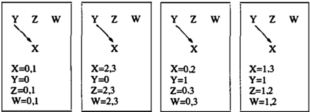
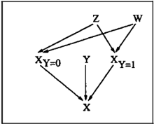
of their values. The use of multiple Bayesian net­ works (Bayesian multinets) are then proposed since contextual strong independence statements cannot be represented naturally in a Bayesian network. For example, consider again the CPT in Table 1. The Bayesian network constructed using the notion of CI does not reflect any independence between variables X and { Z, W} given Y. However, one Bayesian network can be constructed to capture the conditional inde­ pendence of X and {Z, W} given Y = 0, and another to show their dependence when Y = 1 as shown in Figure 1 (left). The particular Bayesian network to be used in the inference process is determined by the evidence.

w

Boutilier et a!. [1] formalized the notion of contex­ tual strong independence with context-strong indepen­ dence ( CSI). ( CSI is called context-specific indepen­ dence in [1].) Let X, Y, C, Z be pairwise dis joint sets of variables. We say X and Z are strongly in­ dependent given Y and the context C = c, denoted I(X j_ Z I Y,C = c), if:

whenever P(Y, C = c, Z) > 0. It should be clear from equation ( 3) that strong CI is a special case of CSI, namely, CSI becomes strong CI when the CSI holds for all c E Vc. That is, if the context-strong independence of X and Z given Y and C = c holds for all c E Vc, then we simply say X and Z are conditionally indepen­ dent given YC. Instead of using Bayesian multinets to capture contextual strong independencies, Boutilier et a!. [1] represent these contextual strong statements with a single Bayesian network by introducing auxil­ iary nodes. Given the CPT in Table 1, the contextual strong independence of variables X and { Z, W} given Y = 0, and dependence when Y = 1, is captured with auxiliary nodes such as X y =O as shown in Figure 1 (right).

In [2], Galles and Pearl studied the notion of prob­ abilistic causal irrelevance (PCI). We say Z is prob­ abilistically causally irrelevant to X given Y if for a fixed y E Vy, the following relationship holds:

Thus, PCI tries to capture the same contextual strong independencies as defined by equation (3). It follows that if the causal irrelevance holds for all y E Vy, then X and Z are probabilistically conditionally inde­ pendent given Y in the usual sense.

It should be clear that the notions of ASI, CSI and PCI all try to capture contextual strong independence, where the partition of the CPT is defined by Y = y. In the next section, however, we introduce a weak contextual independence in which the partition of the CPT is not explicitly defined by the context Y = y.

3 CONTEXTUAL WEAK INDEPENDENCE (CWI)

We now introduce the notion of contextual weak inde­ pendence (CWI), namely, variables X and Z are weakly independent given the context Y = y. We show that this contextual independence is more general than the notions of ASI, CSI, and PCI.

The notions of ASI, CSI and PCI are too strong to capture a weaker form of independence. Let P be a joint probability distribution over the set of vari­ ables U, where X, Y, Z, W E U. Let Vx = {0, 1, 2}, Vy = {0, 1} and Vz = Vw = {0, 1,2,3}. Consider the CPT shown in Table 2, where configurations c with P(c) = 0 are not shown. By equation (1), X and {Z, W} are not conditionally independent given Y. More importantly, there is no contextual strong in­ dependency between variables X and {Z, W} given the context Y = 0 or Y = 1. For example, if Y = O,then

and if Y = 1, then

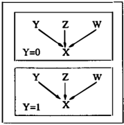
By equations (5) and (6), the notion of ASI does not capture any form of independence between variables X and { Z, W} given Y = 0 or Y = 1 as reflected by the Bayesian multinets depicted in Figure 2 (left). Furthermore, equations (5) and (6) also indicate that variables X and { Z, W} are not contextually indepen­ dent given either the context Y = 0 or the context

P

Y = l. Consequently, the Bayesian network in Figure 2 ( right ) using the notion of CSI by incorporating auxiliary nodes does not reflect any independence between X and {Z, W} given Y = 0 or Y = 1. Figure 2 clearly illustrates that the notions of ASI and CSI do not capture any independency between variabies X and {Z, W} given Y = 0. ( Equations (5) and ( 6) also indicate that variables { Z, W} are not causally irrelevant to X when Y = 0 or Y = 1.)

Table 2: Variables X and {Z, W} are weakly independent given the context Y = 0, but not when Y = 1.

X	y	z	w	P(XIY , Z,W)
0	0	0	0	P1
0	0	0	1	P1
0	0	1	0	P1
0	0	1	1	P1
1	0	0	0	P2
1	0	0	1	P2
1	0	1	0	P2
1	0	1	1	P2
2	0	2	2	P3
2	0	2	3	P3
2	0	3	2	P4
2	0	3	3	P4
0	1	0	0	Ps
1	1	0	2	P6
2	1	1	3	P7

We now informally demonstrate a weak independence between variables X and {Z, W} given the context Y = 0. Let us focus on the configurations (x, Y = 0, z, w ) in Table 2, namely, the set of configurations {t1, t2, . .. , t12}. Recall that the domain of variables X, Y, Z, and W are Vx = {0, 1, 2}, Vy = {0}, and Vz = Vw = {0, 1, 2, 3}. We make a few observations. When Y = 0, only specific values x E Vx appear with specific values z E Vz and w E Vw. That is,

and

In other words, when X = 0 then Z is never 2 or 3 and so forth. Based on this observation let us parti­ tion the CPT in Table 2 into the three separate CPTs {t1,t2, ... , ts}, {tg, tlo, tn, tl2}, and {t13, t14, t14} . Consider the CPT {t1, t2, . . . , t8}. Let us define new domains V.k, Vy, Vz, Vw, based on the values that appear. We obtain

With respect to the new domains in equation (7), by definition variables X and { Z, W} are conditionally independent given Y in the CPT {t1, t2, · · · , ts}. Now consider the CPT {tg, t1o, tu, t12}. Similarly, we define new domains VJ(, V{', V£, V�, for the variables based on the values that appear. Hence,

With respect to the domains in equation (8), however, variables X and { Z, W} are not conditionally indepen­ dent given Y since

We now formalize this idea.

We begin by recalling some familiar notions about re­ lations. Given a distribution P over the set of variables U = XYZ, let

Given any subset V � U, we can define an equivalence relation O(V) on C: for all t;, tiE C,

where tk [V] denotes the value of V in the tuple tk.

Consider two equivalence relations 11(V) and O(W) on T, where V, W � U. The binary operator o, called the composition, is defined by: for t;, tk E T,

if for some ti E T both

Given two equivalence relations 11(V) and O(W) on T, it can be shown that 11(V) o 11( W ) is an equivalence relation ( a partition ) if and only if 11(V) o 11 ( W ) = 11(W) o 11(V). We now define contextual weak inde­ pendence ( CWI ) as follows.

Let X, Y, Z be pairwise disjoint sets of variables in U. Let O(XY = y) and O(Y = yZ) be partitions on C in equation (9). We say variables X and Z are weakly independent given the context Y = y, denoted W I(X l.. ZIY = y), if the following two conditions hold:

• (ii) there exists an equivalence class 1r in O(XY = y) o O(Y = yZ ) such that: for any given x E V�, then for all z E Vz:

where v�, vzr are defined as:

and

Condition (i) says that the composite relation O(XY = y) o O(Y = yZ) is an equivalence relation. This is the necessary condition for W I(X l.. Z I Y = y) to hold. Condition (ii) says that variables X and Z are conditionally independent given Y = y with respect to the new domains v� and vzr.

For example, let us verify that variables X and { Z , W } are weakly independent given the context Y = 0 in the CPT shown in Table 2. By equation (9),

By equation (10), we obtain the following equivalence relations on C:

Applying equation (11), we obtain:

Applying equations (13) and (14) on the configurations 1r1 = {t1, t2, . . . , ts}, we obtain

and

It can be verified that variables X and {Z, W} are conditionally independent given Y = 0 in equivalence class 1r1 with respect to the new domains v;· = {0, 1 } and Vztv = { (0 , 0), (0, 1), (1, 0), (1, 1)}. This pro­ cess can be repeated for the set of configurations 1r2 = {tg, t1o, tu, t12}. The computed new domains are v;, = {2} and Vzw = { (2 , 2), (2, 3), (3, 2), (3, 3)}. As already mentioned, however,

Thus, variables X and {Z, W} are not condition­ ally independent given Y = 0 with respect to the new domains in equivalence class 1r 2. However, con­ dition (ii) is still satisfied since the conditional in­ dependence holds for at least one equivalence class, i.e., 1r1 = {t1, t2, . . . , t s } . By definition, variables X and {Z, W} are weakly independent given the context y = 0.

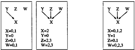
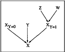
The conditional independence in equivalence class 1r1 is reflected by the Bayesian network in Figure 3 (left). The dependency in equivalence class 1r 2 is reflected by the Bayesian network in Figure 3 (middle). As with ASI and CSI in Figure 2 (left, right), variables X and { Z, W} are not weakly independent given the context Y = 1 as shown in Figure 3 (right).

The important point is that the notion of contextual weak independence (CWI) can capture a more general form of independence than the notions of contextual strong independence. In the above example, the con­ textual strong notions of ASI and CSI do not capture any independence between variables X and { Z, W} given Y = 0 as shown by the various Bayesian net­ works in Figure 2. On the other hand, the notion of

三

二

variables X and Z being weakly independent given the context Y = 0 is captured by the Bayesian network in Figure 3 (left).

4 WEAK INDEPENDENCE (WI)

In this section, we show another important distinction between the notion of contextual weak independence and the contextual strong notions of ASI, CSI and PC I. If the contextual strong independence of X and Z holds for all contexts Y = y, y E Vy, then the notions of ASI, CSI and PCI become strong CI, namely, X and Z are strongly conditional independent given Y. This is not necessarily the case with contextual weak independence. If X and Z are weakly independent for all contexts Y = y, y E Vy, then we say X and Z are weakly independent given Y. Just as contextual weak independence (CWI) is more general than the notions of contextual strong independence (CSI,ASI,PCI), we show that the notion of weak independence (WI) is a more general noncontextual independency than strong Cl. In the next section, we show that the class of WI and CI together has a complete axiomatization.

Let X, Y, Z be pairwise disjoint sets of variables in U. Let B(XY) and B(YZ) be partitions on C in equation (9). We say variables X and Z are weakly independent given Y, denoted W !(X .l Z I Y), if the following two conditions hold:

and (ii) for every equivalence class 1r in the equivalence relation B(YZ) o B(XY), if given any x E Vx, y E V{, then for all z E V{:

where the new domains Vx, V{ and V{ are defined as:

For example, consider the CPT shown in Table 3, where Vx = Vz = Vw = {0, 1, 2, 3 } and Vy = {0, 1 } . Variables X and {Z, W} are not conditionally inde­ pendent given Y. However, variables X and { Z, W} are weakly independent given Y. By equation (9), C = { t1, t2, . . . , t32 }. By equation {1 0 ) , we obtain the equivalence relations B(XY) and B(Y ZW) on C:

Table 3: Variables X and {Z, W} are weakly indepen­ dent given Y.

X	y	Z	W	P(XIY, Z,W)
0	0	0	0	Pl
0	0	0	1	Pl
0	0	1	0	Pl
0	0	1	1	P1
1	0	0	0	Pl
1	0	0	1	Pl
1	0	1	0	Pl
1	0	1	1	Pl
2	0	2	2	Pl
2	0	2	3	Pl
2	0	3	2	Pl
2	0	3	3	Pl
3	0	2	2	Pl
3	0	2	3	Pl
3	0	3	2	Pl
3	0	3	3	P1
0	1	0	0	P2
0	1	0	3	P2
0	1	3	0	P2
0	1	3	3	P2
2	1	0	0	P2
2	1	0	3	P2
2	1	3	0	P2
2	1	3	3	P2
1	1	1	1	P3
1	1	1	2	P3
1	1	2	1	P3
1	1	2	2	P3
3	1	1	1	P4
3	1	1	2	P4
3	1	2	1	P4
3	1	2	2	P4

and

Applying equation {ll), we obtain:

Condition (i) of the definition of WI is then satis­ fied. With respect to the equivalence class 1r1 =

{t1, t2, .. . , t8}, we obtain by equations (20)-(22) the new domains v;·, v;· and v;w:

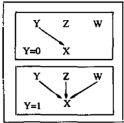
With respect to the new domains v;·, v;· and v;w, variables X and { Z, W } are conditionally indepen­ dent given Y. This conditional independence can be verified similarly in the other equivalence classes 1r2 = {tg, t1Q, . . . ,t16}, 1r3 = {t17,t1s, . .. ,t24}, and 1!" 4 = {t2s, t26 , . .. , ta2}· By definition, variables X and { Z, W} are weakly independent given Y.

There are two equivalent ways to view the represen­ tation of WI. One is in terms of multiple Bayesian networks as in [3]. The difference here is that each Bayesian network has the same dependency structure as shown in Figure 4. As with the Bayesian multinets approach [3], the particular CPT to be used is defined by the evidence. An alternative viewpoint is to rep­ resent WI in a single Bayesian network as with the notion of CSI [1]. The difference here is that no arti­ ficial nodes need to be incorporated into the Bayesian network. Instead each node is simply associated with a set of CPTs compared to a single CPT as with the notion of CI in traditional Bayesian networks.

In the next section, we turn our attention to developing an axiomatic basis for WI.

5 COMPLETE AXIOMATIZATION FOR WI AND CI

There are both theoretical and practical reasons for developing a complete axiomatization for a new type of dependency. When designing a probabilistic net­ work [6], it is always desirable that the designer have complete knowledge about the given input dependen­ cies and all of their logical consequences. On the prac­ tical side, in the absence of knowing a logical conse­ quence, an inference engine may spend precious time on derivations bearing no relevance to the task at hand.

In [ 2] , Galles and Pearl develop axioms to formalize the notion of probabilistic causal irrelevance (PCI) in a similar spirit to the semi-graphoid axioms [6] for Cl. As shown in Section 3, however, the contextual strong notion of PCI is too restrictive to capture contextual weak independence. In this section, we study com­ plete axiomatizations for both the class of weak inde­ pendence (WI) and the class of CI and WI together. Note that we only consider CI and WI statements de­ fined with respect to the same fixed set of variables called nonembedded (full) independencies. That is, we do not consider axioms that involve statements involv­ ing a mixture of variables such as Pearl's contraction axiom (3.6d) [6].

Theorem 1 Let X, Y, Z, W be subsets of variables from U such that XYZ = U. A complete set of infer­ ence axioms for WI is:

Wll, WI2, and WI3 are called reflexivity, transport , and augmentation axioms, respectively. It is interest­ ing to note that there is no transitivity axiom for WI.

Theorem 2 Let X, Y, Z1, Z2 be pairwise disjoint sub­ sets of variables from U such that XYZ1Z2 = U. A complete set of inference axioms for CI and WI to­ gether is:

CI &Wil and CI &WI2 are called weaken and transi­ tivity axioms, respectively.

6 GRANULAR PROBABILISTIC NETWORKS

In this section, we present a brief discussion on granu­ lar probabilistic networks [5]. We use the term granu­ lar to mean the ability to coarsen and refine parts of a

二

probabilistic network. We will show that WI is a nec­ essary and sufficient condition for ensuring consistency in such granular networks.

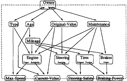
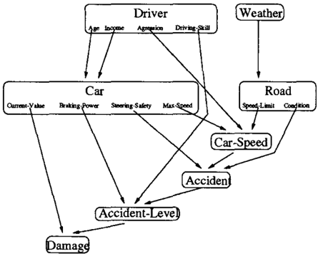
Koller and Pfeffer [5] suggested a framework for the modeling of and inference in a large Bayesian network. In this framework, parts of the network can be coars­ ened and refined. For example, consider the Bayesian network for a car accident [5] as shown in Figure 5. One can refine the node Car to reveal the internal structure as shown in Figure 6, where the rest of the network is not illustrated due to space limitations.

Our purpose here is to present two operators NEST and UNNEST for coarsening and refining a probabilis­ tic network. The main result of this section is that WI is a necessary and sufficient condition for ensuring con­ sistency in such granular networks. (The notion of CI is only a sufficient condition.)

We introduce the operator NEST to coarsen a joint probability distribution. The NEST operator, denoted

N, is used to coarsen parts of a network. Intuitively, NB=Y(Pxy) groups together all the Y-values into a nested distribution given the same X-value.

In the following definitions, we use boldface letters such as t to denote an entire configuration c along with P(c), i.e., t = (c, P(c)). Recall t[X] denotes the value of X in configuration c. The straightforward idea of Nest and Unnest involve rather cumbersome definitions. The examples that follow should clarify any confusion.

Coarsening variables Y in distribution P as at­ tribute B is the distribution NB=Y(P) with variables X, B, P(X, B) defined by

where u E P. The attribute P in the value of B is relabelled P(Y) and the values normalized.

For example, consider the distribution in Figure 7. Coarsening variables {A2, A3} as B is the distribution NB={A,,A,}(P) depicted in Figure 8.

Figure 7: A joint probability distribution P over U = {A1, A2,Aa}.

1	1	2	0.125
1	3	4	0.250
1	5	6	0.125
2	1	3	0.125
2	2	4	0.125
3	0	0	0.125
3	0	1	0.125

We now introduce the operator UNNEST to refine parts of the network. The UNNEST operator, denoted U, reveals the nested variables. Intuitively, U B=Y (P) joins each X-value with each tuple in the correspond­ ing B-value.

Revealing the nested variables Y in attribute B of PxB is the distribution UB=Y(P) with variables XY, P(X, Y) defined by

where u E P, v[X] = u[X], w E v[B] and w[Y] = t[YJ. Note that we may write UB=Y(P) as UB(P) since Y is implicitly implied by B.

For example, revealing the nested variables in coars­ ened distribution P' depicted in Figure 8 results in the refined distribution U B ( P') shown in Figure 7.

Figure 8: The coarser distribution N B={A2,A3} (P) ob­ tained by nesting variables {A2, A3} in the distribution P in Figure 7 as variable B.

	B
1	A2 1	Aa P( A 2 , 2	Aa ) 0.25	0.50
5	3	4	0.50 0.25
1 2 2	A2	6 Aa 3 4	P(A2, Aa) 0.5 0.5	0.25
	A2	Aa	P( A 2 ,Aa ) 0.5	0.25
3	0 0	0 1	0.5

The following example demonstrates that inconsis­ tency may arise due to the fact that the NEST op­ erator is not commutative. (In contrast, the UNNEST operator is commutative.) Consider the distribution Pin Figure 9.

Figure 9: The joint probability distribution P on U = {A1, A2, Aa}.

0	0	0	0.4
1	0	0	0.4
1	0	1	0.2

Suppose we wish to coarsen the variables A1 and Aa. Nesting A3 as Ba followed by A1 as B1 results in the distribution N B,={A.} (N Bs={As} (P)) depicted in Figure 10. On the other hand, coarsening A1 as B1 followed by Aa as B3 results in the distribution NB,={A3}(NB,={A,}(P)) illustrated in Figure 11.

Figure 10: The coarsened distribution NB,={At}(NB3={As}(P)), where P is the joint prob­ ability distribution P in Figure 9.

	B!	A2		Ba	P( B1,A 2 ,Ba )
A! 0	P(A!) 1.0	0	Aa	P(Aa) 1.0	0.6
A!	P( A1 ) 1.0	0	0	P( Aa ) 0.66	0.4
1			Aa 0 1	0.33

Figure 11: The coarsened distribution NB,={A3}(NB,={A.}(P)), where Pis the joint prob­ ability distribution P in Figure 9.

	B!	A2	Ba	P(B1,A2,Ba)
A! 0	P(A1) 0.5	0	Aa P(Aa) 0 1.0	0.8
1	0.5	0	Aa	0.2
A! 1	P( A! ) 1.0		P( Aa ) 0 1.0

We now show that WI is a necessary and sufficient condition for NEST to commute. In other words, WI ensures consistency in granular networks.

Theorem 3 Let P be a joint probability distribution over U, and X, Y, Z pairwise disjoint subsets such that XYZ = U. X and Z are weakly independent given Y if and only if

P ro o f: (:::?) Suppose X and X are weakly independent given Y. By definition, X and Z are conditionally independent given Y in each equivalence class in the equivalence relation II(XY) o II(YZ). One equivalence class is shown in Figure 12, where c = a1 +a2 = b1 +b2 by equation ( 2 ) .

Figure 12: X and Z are conditionally independent given Y in each equivalence class in the equivalence relation II(XY) o II(YZ).

X	Y	Z	P(XYZ)
X!	Yl	Z!	(a1b!}/c
X!	Yl	Z2	(a1b2)/c
X2	Yl	Z!	(azh)/c
X2	Yl	Z2	(a2b2)/c

It is clear that when X and Z are weakly independent given Y, computing NB2=z(P) only groups together tuples in the same equivalence class in the equivalence relation II(XY) o II(YZ). Computing NB2=z(P) mod­ ifies the equivalence class in Figure 12 into the one depicted in Figure 13. The expressions for probability values of B2 can be simplified since, for example

Since the B2-values are identical, computing NB,=x(NB2=z(P)) modifies the equivalence class in Figure 13 into the one illustrated in Figure 14.

二

Figure 13: The distribution NB2=z(P).

Figure 14: The distribution NB,=x(NB,=z(P)).

This demonstrates that each equivalence class in 9(X Y) o 9(YZ) is reduced into a single tuple with all the Z-values and X-values represented in one B1-value and B2-value, respectively. Since the conditional inde­ pendence of X and Z given Y is symmetric, this argu­ ment can be applied to show that NB,=z(NB,=x(P)) also reduces the initial equivalence class in Figure 12 into the single tuple shown in Figure 14. This argu­ ment holds for each equivalence class in the equiva­ lence relation 9(X Y) o 9(YZ).

( ¢) Let P be a distribution such that NB,=x(NB,=z(P)) NB2=z(NB,=x(P)) holds, where one tuple in NB,=x(NB,=z(P)) is depicted in Figure 14. The equality holding indicates that c = a1 + a2 = b1 + b2, as otherwise the order of nesting becomes relevant. The result of UB, (NB,=x(NB2=z(P))) is de­ picted in Figure 13. It can be easily verified that X and Z are conditionally independent given Y in the nor­ malized distribution UB2(UB, (NB,=x(NB,=z(P)))), shown in Figure 15. This argument holds for each tuple in NB,=x(NB2=z(P)). Therefore, X and Z are weakly independent given Y in the distribution NB,=x(NB,=z(P)). D

7 CONCLUSION

Many researchers including (1, 2, 3, 4, 6] have pointed out that the notion of (strong) CI is too restrictive to capture independencies that hold in some but not necessarily all contexts. This kind of contextual inde­ pendency, referred to as context-specific independence (CSI) (1], asymmetric independence (ASI) (3], or prob-

Figure 15: The distribution representing one tuple in UB2(U B, (NB,=x(NB2=z(P)))).

X	y	z	P( X,Y, Z)
Xl	Y1	Zl	b1adc
Xl	Y1	Z2	b2adc
X2	Y1	Zl	b1a2/c
X2	Y1	Z2	b2a2/c

abilistic causal irrelevance (PCI) (2], can be used to facilitate the acquisition, representation, and inference of probabilistic knowledge.

In this paper, we suggest the use of a more general form of contextual independence called contextual weak in­ dependence (CWI) in Bayesian networks. It was ex­ plicitly demonstrated that CWI can detect indepen­ dence that remains undetected by CSI, ASI and PCI. Furthermore, if the contextual strong independency holds for all contexts, then the notions of CSI, ASI and PCI become (strong) CI. On the other hand, if the contextual weak independency holds for all contexts, then CWI becomes weak independence (WI). Just as contextual weak independence ( CWI) is more general than the notions of contextual strong independence, it was explicitly demonstrated that the notion of weak independence (WI) is a more general noncontextual in­ dependency than strong CI. We also studied complete axiomatizations for both the class of WI and the class of CI and WI together. Finally, the interesting prop­ erty of WI being a necessary and sufficient condition for ensuring consistency in granular probabilistic net­ works (5] was demonstrated.

References

• (1] C. Boutilier, N. Friedman, M. Goldszmidt, and D. Koller. Context-specific independence in bayesian networks. In UAI-96, pages 115-123, 1996.
• (2] D. Galles and J. Pearl. Axioms of causal relevance. Artificial Intelligence, 97:9-43, 1997.
• D. Geiger and D. Heckerman. Advances in proba­ bilistic reasoning. In UAI-91, pages 118-126, 1991.
• D. Heckerman and J. Breese. A new look at causal independence. In UAI-94, pages 286-292, 1994.
• D. Koller and A. Pfeffer. Object-oriented bayesian networks. In UAI-97, pages 302-313, 1997.
• J. Pearl. Probabilistic Reasoning in Intelligent Sys­ tems: Networks of Plausible Inference. 1988.