Correlated Action Effects in Decision Theoretic Regression

Craig Boutilier

Department of Computer Science University of British Columbia

Vancouver, BC, CANADA, V6T 1Z4

email:

[email protected]

Abstract

tain problem features are ignored, making certain states in­ distinguishable [8, 3, 11, 5, 16].

Much recent research in decision theoretic plan­ ning has adopted Markov decision processes (MOPs) as the model of choice, and has at­ tempted to make their solution more tractable by exploiting problem structure. One particular al­ gorithm, structured policy construction achieves this by means of a decision theoretic analog of goal regression, using action descriptions based on Bayesian networks with tree-structured condi­ tional probability tables. The algorithm as pre­ sented is not able to deal with actions with cor­ related effects. We describe a new decision theo­ retic regression operator that corrects this weak­ ness. While conceptually straightforward, this extension requires a somewhat more complicated technical approach.

1 Introduction

While Markov decision processes (MOPs) have proven to be useful as conceptual and computational models for deci­ sion theoretic planning (DTP), there has been considerable effort devoted within the AI community to enhancing the computational power of these models. One of the key draw­ backs of classic algorithms such as policy iteration [ 13] or value iteration [2] is the need to explicitly "sweep through" state space some number of times to determine the values of various actions at different states. Because state spaces grow exponentially with the number of features relevant to the problem description, such methods are wildly imprac­ tical for realistic planning problems, a difficulty dubbed by Bellman the "curse of dimensionality."

Recent research on the use ofMDPs for DTP has focussed on methods for solving MDPs that avoid explicit enumera­ tion of the state space while constructing optimal or approx­ imately optimal policies. Such techniques include the use of reachability analysis to eliminate (approximately) un­ reachable states [9, 1 ], and state aggregation, whereby var­ ious states are grouped together and each aggregate state or "cluster" is treated as a single state. Recently, methods for automatic aggregation have been developed in which cer-

In some of these aggregation techniques, the use of standard AI representations like STRIPS or Bayesian networks to represent actions in an MDP can be exploited to help con­ struct the aggregations. In particular, they can be used to help identify which variables are relevant, at any point in the computation of an optimal policy, to the determination of value or to the choice of action. This connection has l e a d to the insight that the basic operations in computing optimal policies for MDPs can be viewed as a generalization of goal regression [5]. More specifically, a Bellman backup [ 2 ] for a specific action a is essentially a regression step where, instead of determining the the conditions under which one specific goal proposition will be achieved when a is exe­ cuted, we determine the conditions under which a will lead to a n u m b er of different "goal regions" (each having dif­ ferent value) such that the probability of reaching any such goal region is fixed by the conditions so determined. Any set of conditions so determined for action a is such that the states having those conditions all accord the same expected value to the performance of a. The net result of this deci­ sion theoretic regression operator is a partitioning of state space into regions that assign different expected value to a. Classical goal regression can be viewed as a special case of this, where the action is deterministic and the value distinc­ tion is binary (goal states versus nongoal states).

A decision theoretic regression operator of this form is de­ veloped in (5). The value functions being regressed are rep­ resented using decision trees, and the actions that are re­ gressed through are represented using Bayes nets with tree­ structured conditional probability tables. As shown there (see also [4]), classic a l g o r ithm s for solving MOPs, such as value iteration or modified policy iteration, can be ex­ pressed purely in terms of decision theoretic regression, to­ gether with some tree manipulation. Unfortunately, the par­ ticular algorithm presented there assumes that actions ef­ fects are uncorrelated, imposing a restriction on the types of Bayes nets that can be used to represent actions.1 The aim of this paper is to correct this deficiency. Specifically, we d e scr i b e the details of a decision theoretic regression al-

1 Correlated effects can be represented by clustering variables, of course, but such a representation is often unnatural and can cause a substantial blowup in representation size.

gorithm that hMdles such correlations in the effects of ac­ tions Md the difficulties that must be dealt with. We note that this paper does not offer much in the way of a concep­ tual advance in the understanding of the decision theoretic regression, and builds directly on the observations in [5, 4]. However, the modifications of these approaches to handle correlations are s ub stant ia l enough, both in technical detail and in spirit, to warrant special attention.

We review MDPs and their representation using Bayes nets and decision trees in Section 2. We briefly describe the ba­ sic decision theoretic regression operator of [ 5) in Section 3. In Section 4, we illustrate the challenges posed by corre­ lated action effects for decision theoretic regres s io n with several examples and describe an algorithm that meets these challenges. We conclude in Section 5 with some remarks on future research and related work.

2 MDPs and Their Representation

2.1 Markov Decision Processes

We assume that the system to be controlled can be described as a fully-observable, discrete state Markov decision pro­ cess [2, 13, 15], with a finite set of system states S. The con­ trolling agent has available a finite set of actions A which cause stochastic state transitions: we write Pr(s, a, t) to de­ note the probability action a causes a transition to state t when executed in states. A real-valued reward function R reflects the objectives of the agent, with R ( s ) denoting the (immediate) utility of being in state s.2 A (stationary) pol­ icy rr : S -t A denotes a particular course of action to be adopted by an agent, with 1r(s) b e i ng the action to be exe­ cuted whenever the agent finds itself in states. We assume an infinite horizon (i.e., the agent will act indefinitely) and that the agent accumulates the rewards associated with the states it enters.

In order to compare policies, we adopt expected total dis­ counted reward as our optimality criterion; future rewards are discounted by rate 0 :=::; f3 < 1. The value of a policy rr can be shown to satisfy [ 13]:

The value of rr at any initial state s can be computed by solv­ ing this system of linear equations. A policy rr is optimal if V" ( s ) 2: V"' ( s ) for all s E S and policies rr'. The optimal value function V* is the same as the value function for any optimal policy.

A number of techniques for constructing optimal policies exist. An especially simple algorithm is value iteration [2). We produce a sequence of n-step optimal value functions vn by setting V0 = R, and defining

2 More general formulations of reward (e.g., adding action costs) offer no special complications.

The sequence of functions vi converges linearly to v· in the limit. Each iteration is known as <1 Bellman backup. Af­ ter some finite number n of iterations, the choice of maxi­ mizing action for each s forms an optimal policy 1r and V" approximates its value.

There are several variations one can perform on the Bell­ man backup. For instance, given a policy rr, we can com­ pute the value of rr by means of successive approximation. If we set V"0 = R, and define

Then V; ( s) denotes the expected value of performing rr, starting at s, fork steps; this quantity converges to V" ( s ) . Finally, given a value function V, we define the Q-function [17], mapping state-action pairs into values, as follows:

This denotes the value of performing action a at state s as­ suming that value Vis attained at future states (e.g., if we acted optimally after performing a and attained v· subse­ quently). We use Qa to denote the Q-function for a particu­ lar action a (i.e., Q a ( s ) = Q ( s, a)). It is not hard to see that value iteration and successive approximation can be imple­ mented by repeated construction of Q-functions (using the current value function), and the appropriate selection of Q­ values (either by maximization at a particular state, or by using the policy to dictate the correct action and Q-value to apply to a state).

2.2 Action and Reward Representation

One of the key problems facing researchers regarding the use of MDPs for DTP is the "curse of dimensionality:" the number of states grows exponentially with the number of problem variables. Since the representation of transition probabilities, reward and value functions, policies, as well as the computations involved in dynamic progr amm ing al­ gorithms, all involve enumerating states, the representation of MDPs and the computational requirements of solution techniques can b e quite onerous. Fortunately, several good representations for MDPs, suitable for DTP, have been pro­ posed. These include stochastic STRIPS operators [14, 3] and dynamic Bayes nets [10, 5]. We will use the latter.

We assume that a set of variables V describes our system. To represent actions and their transition probabilities, for each action we have a dynamic Bayes net (DBN) with one set of nodes representing the system state prior to the action (one node for each variable), another set representing the world after the action has been performed, and directed arcs representing causal influences between these sets. Our con­ vention is to use the notation X' to denote that variable X after the occurrence of the action and X to denote X before the action. Each post-action node has an associated condi­ tional probability table (CPT) quantifying the influence of the action on the corresponding variable, given the value of its influences (see [5, 7] for a more detailed discussion

0

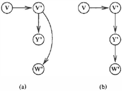
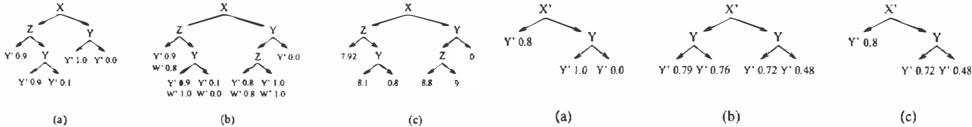
of this representation).3 Figures l(a) and (b) illustrate this representation for two different actions. We use II( X') to denote the parents of node X' in a network and val( X) to denote the values variables X (or X') can take.

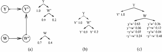
The lack of an arc from a pre-action variable X to a post­ action variable Y' in the network for action a reflects the independence of a's effect on Y from the prior value of X. We capture additional independence by assuming struc­ tured CPTs; that is, we exploit context-specific indepen­ dence (CSI) as defined in [6]. In particular, we use a deci­ sion tree to represent the function that maps parent variable values to (conditional) probabilities. For instance, the trees in Figure l(a) show that Z influences the probability of Y becoming true (as a consequence of the action), but only if X is true (left arrows are assumed to be labeled "true" and right arrows "false"). We refer to the tree-structured CPT for node X' in the network for action a as Tree(X', a). We make special note of the existence of the arc between X' andY' in Figure l(b). This indicates that the effect of ac­ tiona on X and Y is correlated. We will see that such arcs pose challenges for decision theoretic regression.

Finally, a decision tree can also be used to represent the re­ ward function R, as shown in Figure l(c). We call this the (immediate) reward tree, Tree( R). We will also use this rep­ resentation for value functions and Q-functions.

3 Decision Theoretic Regression: Uncorre­ lated Effects

Apart from the naturalness and conciseness of representa­ tion offered by DBNs and decision trees, these represen­ tations lay bare a number of regularities and independen­ cies that can be exploited in optimal and approximate policy construction. Methods for optimal policy construction can use compact representations of policies and value functions in order to prevent enumeration of the state space.

In [5), a structured version of modified policy iteration is developed, in which value functions and policies are repre­ sented using decision trees and the DBN representation of the MDP is exploited to build these compact policies.4 This

3To simplify the presentation, we r es tri c our attention to binary variables in our examples.

4 See [ 12] for a similar, though less general, method in the con-

technique is applied in [ 4] to value iteratio14 and dynamic approximation methods are considered as well. Roughly, if one has a tree representation of a value function, only certain variables will be mentioned as being relevant (un­ der certain conditions) to value. W hen performing Bellman backups, the fact that certain variables are irrelevant to, say, vn means that action-condition pairs that are distinguished by their influence on irrelevant variables need not be distin­ guished in the representation or computation of vn+l.

The key to all of these algorithms is a decision theoretic re­ gression operator used to construct the Q-functions for an action a given a specific value function. If the value func­ tion is tree-structured, this algorithm produces a Q-tree, a tree-structured representation of the Q-function that obvi­ ates the need to compute Q-values on a state-by-state basis. We note that since: (a) the initial value function Tree(R) is tree-structured; (b) the algorithm for producing Q-trees re­ tains this structure; and (c) the algorithm for "merging" Q­ trees (e.g., by maximization) also retains this structure; then the resulting value function will be structured (and meth­ ods for building structured policies based on this can be eas­ ily defined). We focus here only on the construction of Q­ trees-the remaining parts of the algorithms are straightfor­ ward. As in (5, 4], we assume that no action has correlated effects (all have the form illustrated in Figure l(a)): this simplifies the algorithm considerably.

Let a be the action described in Figure l(a), and let the tree in Figure l(c) correspond to some value function V (call it Tree(V)). To produce the Q-function Qa based on V according to Equation 3, we need to determine that the probabilities with which different states s make the condi­ tions dictated by the branches of Tree(V) true.5 It should be clear, since a's effects on the variables in Tree(V) ex­ hibit certain regularities (as dictated by its network), that Qa should also exhibit certain regularities. These are dis­ c overed in the following a l g ori t hm for constructing a Q­ tree representing (the future value component of) Qa given Tree(V) and a network for a.

1. Generate an ordering Ov of variables in Tree(V).
2. Set Tree(Q.,) = 0
3. For each variable X in Tree(V) (using ordering Ov ):
4. (a) Determine contexts c in Tree(V) (partial branches) that lead to an oc­ currence of X.
5. (b) At any leaf of Tree(Qa) such that Pr(c) > 0 fo r some context c: replace the leaf with a copy of Tree( X, a) at that leaf (retain Pr( X) at each leaf of Tree( X, a)); remove any redundant nodes from this copy; for e a c h Y ordered before X such that Pr(Y) labeled this leaf of Tree(Qa), copy Pr(Y) to each leaf of Tree( X, a) just added.

text of reinforcement learning, where deterministic action effects and specific goal regions are assumed).

5 We ignore the fact that states with different reward have dif­ ferent Q-values; these differences can be added easily once the fu­ ture reward component of Equation 3 has been spelled out.

1. At each leaf of Tree( Qa. ) , replace probabilities labeling leaf with I:c Pr(c)V(c), using these probabilities to detennine Pr(c) for any context (branch) of Tree(V).

This decision theoretic regression algorithm forms the core of the policy construction techniques of [5, 4].

We illustrate the algorithm on the example above. We will regress the variables of Tree(V) through action a in the order Y, W (generally, we want to respect the order­ ing within the tree as much as possible). We first regress Y through a, producing the tree shown in Figure 2(a). Notice that this tree accurately reflects Pr(Y') when a is executed given that the previous state satisfies the condi­ tions labeling the branches. We then regress W through a and add the results to any branch of the tree so far where Pr(Y) > 0 (see Figure 2(b)). Thus, Tree(W, a ) is not added to the rightmost branch of the tree in Figure 2(a}­ this is because if Y is known to be false, W has no im­ pact on reward, as dictated by Tree(V). Notice also that be­ cause of certain redundancies in the tests (internal nodes) of Tree(Y, a ) and Tree(W, a ) , certain portions of T re e ( W , a ) can be deleted. Figure 2(b) now accurately describes the probabilities of both Y and W given that a is executed un­ der the listed conditions, and thus dictates the probability of making any branch of Tree(V) true: we simply multiply Pr ( W ) and Pr(Y) for the values of Wand Y labeling this branch. Therefore, the (future component of the) expected value of performing a at any such state can easily be com­ puted at each leaf of this tree using I: { Pr( c) V (c) : c E branches(Tree(V)) } -the result is shown in Figure 2(c).

It is important to note that the justification for this very simple algorithm lies in the fact that, in the network for a, Y' and W' are independent given any context k la­ beling a branch of Tree( Q a ) . This ensures that the term Pr(Y'Ik) Pr(W'Ik) corresponds to Pr(Y', W'lk). There are two reasons for this. First, since no action effects are correlated, the effect of a on any variable is indepen­ dent given knowledge of the previous state (i.e., the post­ action variables are independent given the pre-action vari­ ables). Second, this independence does not require com­ plete knowledge of the state, but can exploit both the vari­ able independence specified by the network structure, and the CSI relations dictated by the CPTs.

4 Regression with Correlated Action Effects

As noted above, the fact that action effects are uncorrelated means that knowledge of the previous state renders all post­ action variables independent. This is not the case when ef-

Figure 3: Dec. theoretic regression: surruning over parents

fects are correlated as in Figure l(b). This can lead to sev­ eral difficulties for decision theoretic regression. The first is the fact that, although we want to compute the expected value of a given only the state s of pre-action variables, the probability of post-action variables that can influence value (e.g., Y') is not specified solely in terms of the pre­ action state, but also involves other post-action variables (e.g., X'). This difficulty is relatively straightforward to deal with, requiring that we sum out the influence of post­ action variables on other post-action variables.

The second problem requires more sophistication. Because action effects are correlated, the probability of the vari­ ables in Tree(V) may also be correlated. This means that determining the probability of attaining a certain branch of Tree(V) by considering the "independent" probabilities of attaining the variables on the branch (as in the previ­ ous section) is doomed to failure. For instance, if both X and Y lie on a single branch of Tree(V), we cannot com­ pute Pr(X'Is) and Pr(Y'Is) independently to determine the probability Pr(X', Y'ls) of attaining that branch. To deal with this, we must construct Q-trees where the joint distri­ bution over certain subsets of variables is computed.

We illustrate the necessary intuitions behind a new algo­ rithm for decision theoretic regression that adequately deals with correlations (i.e., arbitrary DBNs) through a series of examples. We then present the algorithm in its entirety.

4.1 Summing out Post-Action Influences

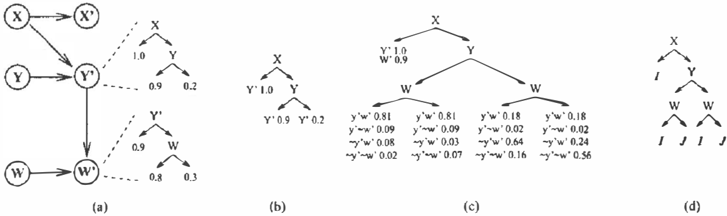
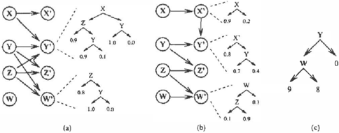
Consider action a in Figure l(b) and Tree(V) in Figure I(c). Using the algorithm from the previous section to produce Tree(Qa), we would first regress Y' through a to obtain the tree shown in Figure 3(a). Continuation of the algo­ rithm will not lead to a legitimate Q-tree, since it involves a post-action variable X'. Our revised algorithm will estab­ lish the dependence of Pr(Y ' ) on previous states by "sum­ ming out" the influence of X' on Y', letting Y' vary with the parents of X'. Specifically, we will simply compute

This will proceed as follows. Once we have regressed Y' through a, we will replace the node X' by Tree(X', a ) . This dictates Pr(X'Ill(X')). Denote the subtree of the

replaced node corresponding to each values x; of X' by STree( x;). Now at each leaf l of Tree (X', a ) just added, we have recorded Pr(xi). For those values of x; that have positive probability, we merge the trees STree( x;) and copy these at l. 6 In Figure 3(b ), we have placed the merged sub­ tree rooted at Y under both X = x and X = :r. Now, at each leaf we can determine (indeed, we have recorded while building the tree) both Pr(X'IX) and Pr(Y'IX', Y) for the appropriate values of X and Y labeling the branch. We can then compute Pr(Y) as needed, depending only on pre-action variables. Once completed, it is easy to see that regression of W' through a can proceed unhindered as in the last section.

We note that had the CPT for X' indicated that Pr( x'lx) = 1 (instead of0.9), we would not have copied the X' = :r' subtree under X = x. This is because the influence of Y on Y' is only valid when X' is false. The result would have been the simpler tree shown in Figure 3(c). Finally, we see that had there been a chain of dependence among post-action variables, this replacement of post-action vari­ ables in the regressed tree by their parents can simply pro­ ceed recursively. For instance, had X' depended on a third variable V', this variable would have been introduced with Tree( X', a ) . The influence of V' on Y' could then have been s unun ed out in a similar fashion.

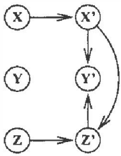
We now consider a second example (see Figure 4) that il­ lustrates that the order in which these post-action variables are replaced in a tree can be crucial. Suppose that we have an action a similar to the one just described, except now we have that variable Y' depends on both X' and Z' (i.e., a's effect on X, Y and Z is correlated). When we regress Y' through a, we will introduce a tree in which both X' and Z' appear, and we assume that X' and Z' appear together on at least one branch of Tree(Y', a ) that is present in Tree( Q a). Now let us suppose that Z' also depends on X', as in Fig­ ure 4. In such a case, it is important to substitute Tree( Z', a ) for Z' before substituting Tree( X', a ) for X'. If we replace X' first, we will compute

(we suppress mention of other parents of Y'). Subse-

6 Merging simply requires c r e a t i n g a tree whose branches make th e distinction contained in each subtree. We do this by order­ ing the trees, and graftin� each tree in order onto the leaves of the tree re s u l t i n g from mergmg it predecessor, and removing redun­ dant nodes (t.e., duplicated tests) as a pp r opriat e.

quently, we would replace occurrences of Z' with Tree( Z') and compute

This ordering has two problems. First, since X' is a parent of Z', this approach would reintroduce X' into the tree, re­ quiring the wasted computation of summing out X' a 7 ain. Even worse, for any branch of Tree(Z') on which X oc­ curs, the computation above is not valid, for Y' is not inde­ pendent of X' (an element ofii(Z')) given Z' and II( X') (since X' directly influences Y').

Because of this, we require that when a variable Y' is re­ gressed through a, if any two of its post-action parents lie on the same branch of Tree(Y'), these nodes in Tree(Y') must be replaced by their trees in an order that respects the depen­ dence among post-action variables in a's network. More precisely, let a post-action ordering 0 p for action a be any ordering of variables such that, if X' is a parent of Z', then Z' occurs before X' in this ordering (so the ordering goes against the direction of the within-slice arcs). Post-action variables in Tree(Y'), or any tree obtained by recursive re­ placement of post-action variables, must be replaced ac­ cording to some post-action ordering 0 p.

4.2 Computing Local Joint Distributions

Consider again Tree(V) shown in Figure l(c) and its regres­ sion through the action a shown in Figure 5(a). Figure 5(b) shows the regression of Y' through a. We would normally then insert Tree(W', a ) at each leaf of this tree, and replace theY' node of this tree with Tree(Y', a ) . Of course, Pr(Y') already labels each leaf, so we can immediately replace the node Y' in Tree(W', a ) with its merged subtrees (as de­ scribed in the previous subsection)? The structure of this tree is indicated in Figure 5(c). If we were to proceed as above, we would simply sum out the influence ofY' on W' to determine Pr(W') at each leaf. That is, we compute

This, unfortunately, does not provide an accurate picture of the probability of attaining the conditions c labeling the branches of Tree(V). If we labeled the leaves of the tree in Figure 5(c) with Pr(Y') and Pr(W') so com­ puted, these probabilities, while correct, are not sufficient to determine Pr(Y', W'): Y' and W' are not indepen­ dent given X, Y, W. Instead, we need the joint distribution Pr( Y ' , W') labeling the leaves, as shown in Figure 5(c). We note that this joint is obtained in a very simple fash­ ion. At each leaf we have recorded Pr(Y') and Pr(W'IY') (under the appropriate conditions). Instead of summing out

7 And as described above, we do not need to include theY' = y subtree (from Tree( W', a)) at the X = x leaf, since Pr(Y') = 1 lab e ls that leaf.

the influence of Y' on W', we explicitly store the terms Pr(Y', W') we compute.8

This approach, explicitly representing the joint probability of different action effects instead of summing out the influ­ ence of in-slice parents, allows us to accurately capture the correlations among action effects that directly impact the value function. We need only compute the joint distribution between two relevant variables in contexts in which they are actually correlated. For instance, sup p ose that v; e sv.:itc�ed the locations of variables Y' and W m T re e ( W , a) m Ftg­ ure S(a). We see then that W' only depends on Y' when W is false. In this case, the final regressed tree (before ex­ pected value is computed) would have a simi.!� shape, as shown in Figure 5( d); but we would compute JOints only at thew-leaves (labeled J). Independent probabilities for Y' and W' can be computed and stored in the usual fashion at the other leaves (labeled J).

The last piece in the puzzle pertains to the decision of when to sum out a variable's influence on an in-slice descendent and when to retain the (local) joint representation. Consider the usual value tree and the action a shown in Figure 6(a); notice that the dependence of W' on Y' has been reversed.

6 We should emphasize that this local joint distribution does not need to be computed or represented explicitly. Any factored representation, e.g., storing directly Pr(Y ' ) and Pr(W ' IY ' ), can be used. In f act, when a number ofvanables are correlated, we gen­ erally expect this to be the approach of choice. However, we will contmue to speak as if the local joint were explicitly represented for ease of exposition.

Regression of Y' leads to the tree in Figure 6(b). When removing the influence of variable W1 on Y', we obtain the tree shown in Figure 6(c). Using the usual ideas from above, we would be tempted to sum out the influence ofW' on Y', computing

However, if we "look ahead," we see that we will later have to regress W' at both leaf nodes for which we are at­ tempting to compute Pr(Y'). Clearly, since these �e.cor­ related, we should leave Pr(Y') uncomputed (exphcttly), leaving the joint representation of Pr(Y', W') as shown in Figure 6(c). When subsequently regressing W' at each . leaf where Pr(Y') > 0, our work is already done at these pomts.

This leads to an obvious question: when removing a P<?St­ action variable V' from the tree produced when regressmg another variable Y' which depends on it, under what cir­ cumstances should we sum out the influence of V' on Y' or retain the explicit joint representation of P r ( V ' , Y')? Intu­ itively, we want to retain the "expansion" ofY' in terms of V' (i.e., retain the joint) if we will need to worry about the correlation between Y' and V' later on. As we saw above, this notion of need is easily noticed when one of the vari­ ables in directly involved in the value tree, and will be re­ gressed explicitly afterward (under the conditions that la­ bel the current branch of course). However, variables that may be needed subsequently are not restricted to those that

have to be regressed directly (i.e., they needn't be part of Tme(V)); instead, variables that influence those in Tree(V) can sometimes be retained in expanded form.

Consider the action in Figure 7(a) (we again use the usual Tme(V)). When we regress Y' through a, we obtain a tree containing node V', which subsequently gets replaced by Tree(V', a ) . The term Pr(Y') should be computed explic­ itly b t sununing the terms Pr(Y'Iv') · Pr(v'IV) over val­ ues v . However, looking at Tree(V), we see that W' will be regressed wherever Pr(Y') > 0, and that W' also de­ pends on V1· This means that (ignoring any CSI) W' andY' are correlated given the previous states. This dependence is mediated by V', so we will need to explicitly use the joint probability Pr(Y', V') to determine the } oint probabil­ ityPr(Y', W'). In such a case, we saythat V isneededand we do not sum out its influence on Y'. In an example like this, however, once we have determined Pr(Y', V', W') we can decide to sum out V' if it won't be needed further.

Finally, suppose that W' depends indirectly on V', but that this dependence is mediated by Y', as in Figure 7(b ). In this case, we can sum out V' and claim that V' is not needed: V' can only influence W' through its effect on Y'. This ef­ fect is adequately sununarized by Pr(Y'IV); and the terms Pr(Y', V'I V) are not needed to compute Pr(Y', W'I V) since W' and V' are independent given Y'. We provide a formal definition of need in the next section.

4.3 An Algorithm for Decision Theoretic Regression

The intuitions illustrated by the previous examples can be put together in an algorithm. We assume that an action a in network form has been provided with tree-structured CPTs (that is, Tree( X', a ) for each post-action variable X'), as well as a value tree Tme(V). We let Ov be an ordering of the variables within Tme( V), and 0 p some post-action or­ dering for a. The following algorithm constructs a Q-tree for Q11 with respect to Tme(V).

1. Set Tree(Qa) = 0
2. 2.
3. For each variable X in Tree(V) (using Ov ) : (a) Determine contexts c in Tree(V) (partial branches) that lead to an occurrence of X. (b) At any leaf l of Tree( Q") such that Pr( c ) > 0 for some contexte, addsimplifY(Tree(X', a), l, k) tol, where k is the context in Tree( Qa) leading to l (we treat las its label).
4. At each leaf of Tree( Qa), replace the probability terms ( of which some may be joint probabilities) labeling t h e leafwtth

Lc Pr( c ) V (c), using these probabilities to determine Pr( c) f or any context (branch) of Tree(V).

The key intuitions described in our earlier examples are part of the algorithm that produces simplify( Tree( X', a ) , l, k). Recall that l is a leaf of the current (partial) Tree( Q") and is labeled with (possibly joint) probabilities of some sub­ set of the variables in Tree( V). Context k is the set of con­ ditions under which those probabilities are valid; note that k can only consist of pre-action variables. Simplification involves the repeated replacement of the post-action vari­ ables in Tree( V) and the recording of joint distributions if required. It proceeds as follows:

1. Reduce Tree( X', a ) f or context k by deleting redundant nodes.
2. For any variables Y' in Tree( X', a) whose probability is p art of the label f or l, replace Y' in Tree( X', a ) , respecting the ordering 0 p in replacement. That is, for each occurrence of Y' in Tree( X', a ) :
3. (b) compute Pr(X'[Y', m ) · Pr(Y') for each leaf in the merged subtree (let this leaf correspond to context m = k II k', where k' is the branch through Tree( X', a));
4. (a) merge the subtrees under Y' corresponding to values y of Y' that have positive probability, deleting Y';
5. (c) if Y' has been regressed at l or is needed in context m, la b el this leaf of the merged tree with the joint distribution over X', Y'; otherwise, sum out the influence of Y'.
6. For any remaining variables Y' in Tree( X', a ) , replace Y' in Tree( X', a), respecting ordering Op in replacement; i.e., (a) replace each occurrence of Y' with Tree(Y', a) (and re­ duce by context n = k II k', where k' is the branch through Tree( X', a) leading toY ' ); ) just added, merge the that have
7. (b) to each leaf l' of the Tree(Y', a subtrees under Y' corresponding to values y of Y' positive probability at l'; (c) proceed as in Step (2).
8. Repeat Step 3 until all new post-action variables introduced at each iteration of Step 3 have been removed. For an y vari­ able removed from the tree, we construct a joint distri b ution with X' if it is needed, or sum over its value if it is not.

These steps embody the intuitions described earlier. We note that when we refer to Pr(Y') as it exists in the tree, it may be that Pr(Y') does not label the leaf explicitly but jointly with one or more other variables. In such a case, when we say that Pr(X', Y') should be computed, or Y' should be sununed out, we intend that X' will become part of the explicit joint invo I ving other variables. Any variables that are part of such a cluster are correlated with Y' and hence with X'. Variables can be summed out once they are no longer needed.

The last requirement is a formal definition of the concept of need-as described above, this determines when to retain a joint representation for a post-action variable that is being removed from Tree(Q11). Let l be the label of the leaf where X' is being regressed, k be the context leading to that leaf, Y' be the ancestor of X' being replaced, and k' the context labeling the branch through (partially replaced) Tme( X', a ) where the decision to compute Pr(X') or Pr(X', Y') is be­ ing made. We say that Y' is needed if:

• 1 . there is a branch b of Tree( V) on which Y' lies, such that b has positive probability given I ; or
• there is a branch b on which Z lies, such that b has pos­ itive probability given l; Pr(Z' ) is not recorded in l; and there is a path from Y' to Z in a's network that is not blocked by {X', k, k' } .

5 Concluding Remarks

We have presented an algorithm for the construction of Q­ trees using a Bayes net representation of an action, with tree-structured CPTs, and a tree-structured value function. This forms the core of a decision theoretic regression algo­ rithm. Unlike earlier approaches to this problem, this al­ gorithm works with arbitrary Bayes net action descriptions, and is not hindered by the presence of "intra-slice" arcs in the network reflecting correlated action eff ects. This is an important feature because this representational power al­ lows one to concisely represent actions in a natural fashion. Forcing someone to specify actions without correlations is often unnatural, and the translation into a network with no intra-slice arcs (e.g., by clustering variables) can cause a blowup in the network size and the inability to exploit many independencies in decision theoretic regression.

One concern about such approaches is the overhead in­ volved in constructing appropriate trees. We note that this algorithm will behave exactly as the algorithms discussed in [5, 4] if there arc no correlations. While we expect MDPs to often contain actions that exhibit correlations, it seems likely that many of these correlations will be localized. Fur­ thermore, the usc of context-specific independence allows clustering to be perf ormed only under the specific condi­ tions that give rise to the dependencies among effects. Fi­ nally, we observe that we are only concerned with main­ taining correlations among variables that actually influence value. If we are dealing with effects that impact other rele­ vant effects, but are not of direct interest themselves, these are summed out immediately with little overhead.

We are currently exploring the extent to which networks can be preprocessed to alleviate some of the repeated operations at different regression steps. There is also an interesting connection to the recent work ofMichael Littman (personal communication); he has suggested the transformation of ac­ tion representations such as ours into a S TRIPS representa­ tion of actions that does not require correlated effects to be represented explicitly. This is achieved by a radical trans­ formation of the problem, but one that is polytime, requires only a polynomial size increase, and from which an optimal policy can be extracted in polynomial time. It is an open question ifthat method exploits the same type of structural regularities as our approach. Finally, we hope to consider the use of other compact CPT representations in decision theoretic regression.

Acknowledgements

This research was supported by NSERC Research Grant OGP0121843 and IRIS NCE Program IC-7.

References

• [ I ] A. G. Barto, S. J. Bradtke, and S. P. Singh. Learning to act us­ ing real-time dynamic programming. Artificial Intelligence, 72(1-2):8 1-1 38, 1 995.
• [2} Richard E. Bellman. Dynamic Programming. Princeton Uni­ versity Press, Princeton, 1 957.
• [3} Craig Boutilier and Richard Dearden. Using abstractions for decision-theoretic planning with time constraints. In Pro­ ceedings o f the T welfth National Conf erence on Artificial In­ telligence, pages I 016-1 022, Seattle, 1 994.
• Craig Boutilier and Richard Dearden. Approximating value trees in structured dynamic programming. In Proceedings o f the Thirteenth International Con f erence on Machine Learn­ ing, pages 54--62, Bari, Italy, 1 996.
• Craig Boutilier, Richard Dearden, and Moises Goldszmidt. Exploiting structure in policy construction. In Proceedin � s o f the Fourteenth International Joint Con forence on ArtiJl­ cia! Intelligence, pages I I 04-l l l \, Montreal, 1 995.
• [6} Craig Boutilier, Nir Friedman, Moises Goldszmidt, and Daphne Koller. Context-specific ind � p endence in Bayesian networks. In Proceedings o f the T we/j th Con f erence on Un­ certainty in Artificial Intelligence, pages 1 1 5--1 23, Portland, OR, 1 996.
• Craig Boutilier and Moises Goldszmidt. The frame problem and Bayesian network action representations. In Proceed­ ings o f the Eleventh Biennial Canadian Con f erence on A rti­ ficial Intelligence, pages 69-83, Toronto, 1 996.
• David Chapman and Leslie Pack Kaelbling. I n p u t general­ ization in delayed reinf orcement learning: An algorithm and performance comparisons. In Proceeding s o f the T welfth In­ ternational Joint Conforenceon Artificial I ntelligence, pages 726-73 1 , Sydney, 1 99 1 .
• Thomas Dean, Leslie Pack Kaelbling, Jak Kirman, and Ann Nicholson. Planning with deadlines in stochastic domains. I n Proceedings o f the Eleventh National Con forenceon Arti­ ficial Intelligence, pages 574-579, Washington, D.C., 1 993.
• [ 1 0] Thomas Dean and Keiji Kanazawa. A model f or reason­ ing about r e r sist e nc e and causation. Computational Intel­ ligence, 5{3): 1 42-1 50, 1 989.
• [ I I ] Richard Dearden and Craig Boutilier. Abstraction and ap­ proximate decision theoretic planning. Artificial Intelli­ gence, 1 996. To appear.
• [ 1 2] Thomas G. Dietterich and Nicholas S. Flann. Explanation­ based learning and reinforcement learning: A unified ap­ proach. In Proceedings o f the T welfth International Con­ ference on Machine Learning, pages 1 76-1 84, Lake Tahoe, 1 995.
• [ 1 3} Ronald A. Howard. D ynamic Programming and Markov Processes. MIT Press, Cambridge, 1 960.
• [ 1 4] Nicholas Kushmerick, Steve Hanks, and Daniel Weld. An algorithm f or probabil istic \east-commitment planning. In Proceedings o f the T welfth National Con forenceon Artificial Intelligence, pages I 073--1 078, Seattle, 1 994.
• [ 1 5 ] Martin L. Puterrnan. Markov Decision Processes: Discrete Stochastic Dynamic Programming. Wiley, New York, 1 994.
• [ 1 6} John H. Tsitsiklis and Benjamin Van Roy. Feature-based methods for large scale dynamic programming. Machine Learning, 22:59-94, 1 996.
• [ 1 7] Christopher J. C. H. Watkins and Peter Dayan. Q-learning. Machine Learning, 8:279--292, 1 992.