Decision Theoretic Foundations of Graphical Model Selection

Paola Sebastiani

Department of Actuarial Science and Statistics City University

Abstract

This paper describes a decision theoretic for­ mulation of learning the graphical structure of a Bayesian Belief Network from data. This framework subsumes the standard Bayesian approach of choosing the model with the largest posterior probability as the solution of a decision problem with a 0-1 loss func­ tion and allows the use of more general loss functions able to trade-off the complexity of the selected model and the error of choos­ ing an over-simplified model. A new class of loss functions, called disintegrable, is in­ troduced, to allow the decision problem to match the decomposability of the graphical model. With this class of loss functions, the optimal solution to the decision problem can be found using an efficient bottom-up search strategy.

1 INTRODUCTION

A Bayesian Belief Network (BBN) is defined by a a joint probability distribution over a directed acyclic graph (DAG), where nodes represent stochastic variables and arcs identify dependencies between a set of parent vari­ ables and a child variables. The independence assump­ tions embedded in the graph factorize the joint prob­ ability distribution into a set of conditional distribu­ tions, so that reasoning tasks can be efficiently per­ formed. Although in their original formulation, both the graphical structure and the conditional probability distributions were supposed to be provided by domain experts, for the last ten years learning BBNs from data has been an active field of research. There are now several techniques to extract the graphical model of a BBN from data (Cooper and Herskovitz, 1992; Beck­ erman, 1997; Lauritzen, 1996; Whittaker, 1990) and BBNs are becoming an important tool in several rna-

Marco Ramoni

Knowledge Media Institute The Open University chine learning and data mining applications. Among statistical techniques, Bayesian methods have the ad­ vantage of coupling expert knowledge on the domain of application with the sample information in the learn­ ing process. The standard Bayesian approach to model selection involves three distinct operations:

1. A set of possible models is identified, with their prior probabilities representing the expert belief in the ability of the models to capture the association among the variables.
2. A random sample of cases is collected, which is used to update the prior probabilities of each model into posterior probabilities, by using Bayes' Theorem.
3. The model with the largest posterior probability is selected.

The rationale behind this strategy is that the model with the largest posterior probability is the most likely on the light of the sample information. It is evident that model selection involves a decision process and therefore decision theory can be used to provide a nor­ mative foundation for it (Berger, 1985; Savage, 1972). Since the decision to be made concerns the statistical problem of selecting a model on the basis of its prior probability and information conveyed by data, the de­ cision problem is usually referred to as a statistical de­ cision problem (Berger, 1985). The decision theoretic formulation of the model selection process subsumes the standard Bayesian strategy of selecting the model with the largest posterior probability as the solution of a decision problem with a 0-1 loss function. Further­ more, it allows the use of different loss functions able to trade-off the complexity of the selected model and the error of choosing an over-simplified model, thus taking into account features of the extracted model that are important for the subsequent use made of it.

Although, in principle, the formulation and solution of this decision problem seems to be immediate, we are faced with the problem that, as the number of vari­ ables increases, a complete enumeration of all models

is not feasible, and the formulation of the loss func­ tion can be too difficult. The complexity of the search in the model space is also a problem for the standard Bayesian strategy, which is typically overcome ( Cooper and Herskovitz, 1992) by reducing the model selection process to a greedy search over a subset of models which are consistent with some order among the vari­ ables. We show that this strategy can be formulated as a sequential decision problem and we introduce a new class of loss functions called disintegrable that de­ compose the sequential decision problem into smaller independent problems which admit, as optimal, an ef­ ficient one-step-look-ahead strategy.

Next section formulates the selection of the DAG of a BBN as a decision problem, and it shows how the stan­ dard Bayesian approach to model selection is equiv­ alent to the solution of a statistical decision problem with a 0-1 loss function. Section 3 describes the se­ quential decision approach to greedy model search, and its solution when the loss function is disintegrable is given in Section 4.

2 NORMATIVE MODEL SELECTION

In order to introduce the decision theoretic approach to model selection, we begin by considering a simple discrimination problem between two DAGs and then we will generalize the results to an arbitrary number of models.

2.1 MODEL DISCRIMINATION

Suppose we have two categorical variables X1 and X2, and a random sample 1) of n cases. The task is to discriminate between two DAGs: Mo specifies that X1 and X2 are independent variables, M1 specifies that X2 is a parent variable of X1. The standard Bayesian solution to this problem is to assign prior probabilities p(Mo) and p(Ml), use the available data to compute the posterior probabilities p(M0jV) and p(M1j1J) and then choose the model with the largest posterior prob­ ability. Given that:

where p(V) is the marginal probability of the data, and p(V jM;) is the marginal likelihood, the model selection is based on the value of the ratio

from which the following decision rule is derived: if r < 1, M1 is chosen, if r > 1, M0 is chosen, and

•o

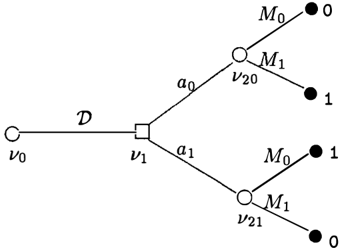
Figure 1: Decision tree for the decision problem with 0-1 loss function

if r = 1 then the two models are equivalent. When p(Mo) = p(Ml), r is the Bayes factor, i.e. r = p(VIMo)fp(VjMl)·

Within this formulation, the discrimination between Mo and M1 reveals to be a statistical decision prob­ l em in which the true state of Nature is an element of the set M = {Mo, Ml}, the action space A is the set { ao, al}, where a; is the action "choose Mi'' , data is the sample V, and the l oss function is the 0-1 function defined for (M, a) EM x A as:

The decision problem is represented by the decision tree in Figure 1, in which circles represent random nodes, squares represent decision nodes, and leaves ( black circles ) are value nodes. Thus, we first collect data V, then use the data to choose either action a0 or a1. The loss incurred if the true state of Nature reveals to be M; and the action chosen is aj is then represented in the leaf nodes, and it is 1 if i =j:. j and 0 otherwise. The optimal decision, i.e. the Bayesian action, is found by minimizing the expected loss. This is done by "averaging out" and "folding back" ( Raiffa and Schlaifer, 1961). From the terminal nodes, we compute the expected loss at random nodes, given ev­ erything on the left of the node, and we minimize the expected loss at the decision nodes. The expected loss of the decision a;, also known as the risk of the decision a;, at the node v2;, is

where the expectation is over the conditional distribu­ tion of M given 1). The Bayesian action is found at

node liz by choosing:

which is equivalent to the decision rule r found above. The risk of the Bayesian action is called the Bayesian risk and it is the posterior probability of the model chosen.

This formalization has the advantage that we can gen­ eralize the decision problem by using different loss functions, without modifying the prior probabilities of Mo and Mt. The 0-1 loss function penalizes the choice of an unnecessary complex model (Mt instead of Mo) as the choice of an over-simplified model (Mo instead of Mt). In general, we may wish to penalize the two errors in different ways, and this can be done by using

the 0-L loss:

Thus, l;j is the loss incurred if the state of Nature is represented by model M; and model Mj is chosen. In this case, the risks at vzo and llzt are

and, therefore, the Bayesian action is at if p(Mti1J) > lotP(Moi1J)/lto or, equivalently, if p(1JIMt) > (lotP(Mo)p(1JIMo)) / (ltop(Mt)).

Example 1 Let Xt be a discrete variable with Ct states, and let X2 be a discrete variable with c2 states. For simplicity we will denote the events Xz == Xzj and Xt == X!k by Xzj and Xtk· Model Mo specifies that the two variables are independent and, condi­ tional on M0, we can parameterize p(x2jiB ( 0 ) ) == Bj and p(XtkiB ( 0 ) ) == O .k . Thus, (;l ( O) is the parameter vector associated to Mo. Model Mt specifies that X2 is a par­ ent of Xt, and the associated parameter vector (;l ( t ) has elements Bj == p(x2jiB ( t ) ) and p(xtkiX2j, (;l ( t ) ) == Bjk· It is well known ( see for instance the recent review by Heckerman ( 1 997)) that the marginal likelihood p(1JIM;) is easily found under the assumptions that: 1. the sample is complete; 2. the cases are independent, given the parameter vector O(i) associated to M;; 3. the prior distribution of the parameters is a Dirichlet distribution; 4. the parameters are marginally inde­ pendent.

Suppose that, given Mo, BJ = (Bt, ... , Bc 2) "' D(a/c2, ... ,ajc2) and O.K = (B.t, ... , B. c J D(afct, ... , afct), where D(at, ... , an) is a Dirichlet distribution with hyper-parameters (at, ... , an)· Given Mt, we assume that BjK = (Bjt, . . . , Bj c J "' 2

D(a/(ctc2), ... , a/(ctc2)). These parameterizations ensure that, a priori, the probabilities p(x2j), p(xlk) and p(XtkiXzj) are all uniform and are based on the same total prior precision on (;l(i). Let n(xlklx2j) be the sample frequency of (XtkiX2j), so that n(x2j) == 2::�� 1 n(x1kiX2j) is the sample frequency of X2j, and n(xlk) == I:j�t n(x1kiX2j) is the sample frequency of Xtk· Then:

and the Bayesian action under a general 0-L loss func­ tion is to choose model Mt if

If the effect of the prior hyper-parameters is negligible, for instance when the frequencies n(xtkiX2j) are large, and p(Mo) == p(Mt), then r is equivalent to the likeli­ hood ratio test (Berger, 1985 ) , and the Bayesian rule becomes equivalent to the classical significance test. In this case, Mo is accepted if 2 logr < x ! , (c t -t )(c2 -t ) ' where x ! , ( c 1 -t )( c 2t ) is the (1 - a)% quantile of a x 2 distribution on ( Ct - 1) ( c2 -1 ) degrees of free­ dom. Thus, when 2 ( log ltoP{Mt) - loglotP(Mo)) == x ! , ( ctt ) ( c2 -t ) the decision rules in both approaches are identical. Note that, in the classical approach, the region of the sample space in which Mt is rejected as true model, is a function of the number of states of the variables Xt and x2. 0

2.2 GENERAL SOLUTION

The framework described in the previous section can be generalized to the situation in which we have a set of variables X== {Xt, · · · , X1 }, and we look for a DAG to represent the independence assumptions among the variables. Let M == {M0, Mt, . .. , Mg } be the set of all possible models, representing the possible states of Nature. We will keep the symbol M0 to denote the null model: the model of mutual independence among the variables in X. These g + 1 models determine the action space which is now A == { a 0 , at, . . . , a g } , and

the action a; represents the choice of model M;. The loss function is given by a ( g + 1) x ( g + 1) table:

where l;j is the loss incurred if the true state of Na­ ture is M;, and Mj is chosen. The larger number of possible models induces an expansion of the decision tree in Figure 1. Node v1 will have g + 1 branches, each of them corresponding to one of the possible ac­ tions. Each branch corresponding to the action aj will terminate in a random node v2j corresponding to the "revelation" of the true state of Nature and it will then be expanded into g + 1 branches repre­ senting the possible states of Nature. Thus, at the leaves of each branch there will be the loss incurred: l;j, i = 0, . . . ,g. The Bayesian action a* is then found by minimizing the expected loss. The risk of the ac­ tion aj at node v2j is R(aj,'D) = L:f =0 l;jp(M;IV) and a* = arg min;{R(aj, V)} . With a 0-1 loss func­ tion, the Bayesian action corresponds to the standard Bayesian solution.

Theorem 1 For the decision problem with data V, state of Nature M = {Mo, M1, ... , M9 } , action space A= { a0, a1, ... , a9 } , where a; is the choice of M;, and loss function defined as in {1}, with l;j = 1 fori # j, the Bayesian action is a; if p(M;IV) > p(Mji'D) for all j # i.

Proof. It is enough to show that R(a;, V) R(aj, V) < 0 for all j # i. Suppose that p(M;!V) > p(Mji'D) for all j # i, then R(a;,V)- R(aj,'D) p(Mji'D)- p(M;IV) < 0 for all j # i. D

With a generic loss function, however, the Bayesian action may not be so simple to identify.

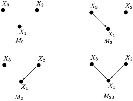
Example 2 Let X = {X1, X2, X3 } and denote by c; the number of states of X;. Suppose that X2, X3 are known to be marginally independent, and that they can be both parents of xl, but xl cannot be parent of X2, X3. The set of possible models to be considered is limited to M= {Mo, M2, M3, M23 } which are given in Figure 2. Thus, the action space is given by the four possible actions of choosing one of the four models. Suppose we use the loss function L(M, a) =

Figure 2: Models in Example 2.

	ao	a3	a2	a23
Mo	0	kc3	kc2	k(cg+ c2)
M3	h	0	k(c3+ c2)	kc3	(2)
M2	h	k(c3+ c2)	0	kc2
M23	2h	h	h	0

where h and k are positive constants. Thus, the loss for choosing an unnecessarily complex model is an in­ creasing function of the number of states of the vari­ ables. On the other hand, the loss for the choice of an over-simplified model is an increasing function of the number of possible parents left. The four risks are:

and the Bayesian action is the one with minimum risk. Suppose, for instance, that p(M3ID) = p(M2ID) = p, p(M23ID) = 2p and p(Mo!D) = 1- 4p, with p < 0.25. Suppose further c3 = 2 and c2 = 3. Then,

We have R(ag, 'D) < R(a2, V), so that M3 is preferred to M2, although the two models have the same poste­ rior probability. A 0-lloss function would not allow us to discriminate between M2 and M3 · Note also that R(a3, V) = 2k- 3kp+ 2hp � 5k - 15kp = R(a23, 'D) if p � 3k/(12k + 2h). Since 3k/(12k + 2h) < 0. 25, then R(ag, V) < R(a23, V) if p < 3k/(12k + 2h). Further­ more, we have the following inequalities:

15k

> 8h

Figure 3: Ordering among risks for Example 2 when 0 < p < 0.25: Ro = R(ao, 'D); Rs = R(as, 'D); R2s = R(a23, 'D).

The ordering among risks given in Figure 3 induces the following decision rule:

If 15k ::; 8h then

If 15k > 8h, then

Thus, the standard Bayesian solution of choosing model M23, is replaced by a more complex strategy, in which model M23 is chosen if its probability is larger than 3k/(6k +h ) . In other word, a complex model is chosen when there is enough evidence in favor of it.

A simpler loss function would yield a simpler decision rule. Suppose, for instance, that we decide to penalize the choice of a complex model uniformly, via the loss function:

		ao	as	a2	a23
	Mo	0	1	1	1
L(M,a)=	Ms	h	0	h	h
	M2	h	h	0	h
	M2s	2 h	2 h	2h	0

The risks of the four actions are:

For instance, a0 is the Bayesian action if Po > hps, Po > h p2 and Po > 2hp23: the null model is chosen if its posterior probability is h-times larger than the posterior probabilities of the two models with one arc only, and twice as large as the posterior probability of the model with two arcs. In doing so, we let the choice of the model depend on the complexity of the network to be chosen, and we favor the choice of more complex models. Note that the comparison between models Ms and M2 depends only on their posterior probabilities, and it is therefore consistent with this strategy, since both models have the same number of arcs. D

Clearly, as the number of variables increases, so does the complexity of the decision problem to solve, and we are faced with two problems:

(1) The definition of the loss function becomes too complex.

1. The number of possible models explodes.

Problem (2) has been examined by several authors, and a solution is to reduce the model selection pro­ cess to a greedy search over a subset of models which are consistent with some order among the variables, by taking advantage of the multiplicative form of the pos­ terior probability of a model. We can similarly decom­ pose the decision problem into sub-problems to match the decomposition of the model search.

3 DECOMPOSABLE DECISION PROBLEMS

Suppose we have an order on the variables in X {X1, ... ,Xr } , so that X; � Xj if X; cannot be par­ ent of Xj. Let P; = { X;1, ... , X; qJ be the set of possible parents of X;. Thus, P; is the empty set if X; is a root node. Consider a DAG M, that spec­ ifies, for each node variable X;, the set of its par­ ents, and let them be II;. Denote by n(x;kJ1r;j), i = 1, ... ,I, j = 1, ... , �CJi, k = 1, . . . , c;, the sample fre­ quency of (x;k, 11" i j), so that n(?r i j) = I:% ;= 1 n(x;kJ 1r;j) is the sample frequency of 11" i j. We also invoke As­ sumptions 1 4 listed in the description of Exam­ ple 1 and assume that, given M, the vector of pa­ rameters B;j = ( B;j 1, ·.. , B ;j c; ) associated to the con­ ditional distribution of X; J 7r ;j has a Dirichlet distri­ bution D(a i j l , ... , O: i jc;)· Thus, a;j = L:k O: i jk is the prior precision of B;j. It is shown by Cooper and Her­ skovitz (1992) that the posterior probability of M is

Note that p(MJV) has a multiplicative structure, since p(MJV) is given ( up to a proportionality constant ) by the product, over the sets {X;, P i }, i = 1, ... , I, of the

probabilities

associated to the local dependencies in {X;, P;}. This property is exploited by Cooper and Herskovitz (1992) to derive a bottom-up search strategy over the sets {X;, P ; } known as K 2 algorithm. In order to capture this search strategy in a decision theoretic framework, we need to define an algebraic structure on the set of models. Let Mi be the set of possible models to be explored in each {X;, P;}. This set can be represented by a matroid with q; + 1 levels. Each level contains ( q; ) C(q;,j) = j models with j arcs pointing to X;. We shall denote one such a model by M�o ( q ; , j ) ' where co ( q;, j) is a possible combination of j indexes out of the q; indexes i1, i2, ... , iq; that identify the variables in P;. The number of models to be explored in Mi . th 2 q ' - "' q ' ( q; ) L t M ; M ; Mi b IS en - L.. j = l j . e 0, 1 , ... , q ; e elements of Mi where M� is the null model, and each Mj is the model with only one arc from X;j point­ ing to X;, We can regard the set Mi as generated by M&, Mf, ... , M�, via the sum of models l±J which is defined as follows. Let M�o ( q ; , j ) and M�o(q ; ,l ) be ele­ ments of M;, then M�o ( q ; , j ) l±J M�o ( q; , l ) = M�o (q ;, m ) is the model containing all arcs pointmg to X;, that are specified by the two models. This algebraic structure decomposes every model with more than one arc point­ ing to X;, into the sum of models with one arc only, Mi Mi ·�· M i ·�· ·�· M l D · t . th e.g. i l , . . . , i k = 06 1 6 ... 6 k . .t·or ms ance,m e four models in Figure 2, M23 is the sum M2l±JM3. Fur­ thermore, if M�o(q ; ,j ) and Mfo(q j ,l ) are models in Mi . . j and MJ, we define M�o(q ; ,j ) l±J M c o(q j , l ) as the model containing all arcs specified by the two models. In this way, every DAG for the variables in X can be regarded as a sum of models in Mi, i = 1, . . . , I.

The decision problem describing the search over the sets Mi is now a pseudo sequential statistical decision problem: we use the term "pseudo" because we do not have a sequential collection of data. A typical branch of the decision tree is represented in Figure 4. Once

data are collected at node vo, at node v1 we choose an action from the action space A 1 = { a a, a � , ... , a�q1 }, corresponding to all possible models M1. The conse­ quence of each action is represented by the possible models in M1. Next, we have the decision node v2 with action space A 2 = { a 6 , a i , ... , a � q2 } , correspond­ ing to a choice in the set M2. The consequence of each action is represented by the possible models in M2, and so on. The decision problem terminates after I steps, corresponding to the I sets Mi. It is evident that we can regard each action space Ai as generated by a t , a i , ... , a � , , with a � defined as choosing model Mj. The choice of a model with more than one arc is then the sum of the generating actions, i.e. a � 1 = a� l±J a } is "choose the models with arcs from X;j and from X i !" and so on. The terminal nodes in the decision tree report the loss incurred when the true state of Nature correspond to the sum of models "revealed" along the branch, and the action chosen is the sum of actions taken at the I decision nodes in the branch. As in Section 2, the problem is solved by averaging out and folding back. Thus, we start from the terminal nodes in the tree, we find the action that minimizes the ex­ pected loss given everything is on the left, and then we proceed backward, by finding optimal actions and folding back the tree. The decision nodes are replaced by value nodes reporting the Bayesian risks of the op­ timal actions. Next section will show that, in our case, there exists a class of loss function which admit a so­ lution easy to find.

4 DISINTEGRABLE LOSS FUNCTIONS

The algebraic structure on the set of all possible mod­ els translates into a similar structure on the loss func­ tion. Consider first the local decision problem in Mi. The loss function can be built up from simple loss functions associated to the q; pair-wise comparisons between M& and each Mj as follows. Let L� (Mi, a i ) be the 0-L loss function for discriminating between models M& and Mj, were a � is the action "choose model Mj". Thus, L� (Mi, a i ) is defined over the space {Mj,Mj} X { a t ,a n as:

We define the sum EEl of L � ( Mi , a i ) and L f ( Mi , a i ) as the loss function defined over the set [ { Mj, Mj } l±J

	a h	aj	a• I	a j l
M6	0	loj	lot	l o j + l o t
Mi J.	ljo	0	lot +ljo	lot
M' I	Ito	l10 + loj	0	l o j
Mjl	ljo +l10	liD	ljo	0

By iteratively computing the sum of all q; loss func­ tions, we derive the loss function for the local decision problem in M i which is defined on M i x A i :

We will call a loss function which can be obtained in such a way a locally disintegrable loss function.

The rationale behind the choice of this loss function is that the error in choosing M:o(q; , j) instead of Mfo ( q ; , l) is in the number of arc differences between the two models and we penalize this error by summing up the losses corresponding to each arc difference. Consider, for instance, the four models in Figure 2. The error in choosing either models M3 or M2 compared to Mo is only in one arc. If M2 is chosen instead of M3, the error is given by adding the arc from X2 to X1 ( i.e. choosing M2 instead of Mo) and removing the arc from X3 to X1 ( i.e. choosing M0 instead of M3.) We thus penalize this error by summing up the two losses corresponding to choosing M2 instead of M0, and to choosing M0 instead of M3.

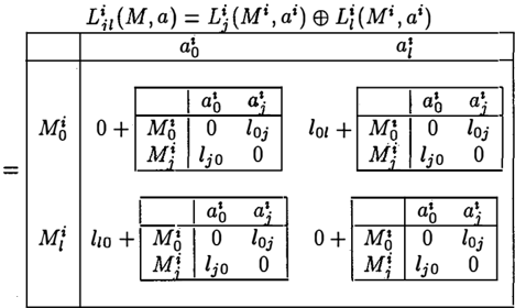
Let now Li(M,a), i = 1, ... ,!, be the disintegrable loss functions associated to the I local decision prob­ lems. We define as globally disintegrable for the se­ quential decision problem the loss function generated as:

Thus, L(M, a) is a table of dimensions fl; 2q; x TI; 2q;. Ea-ch row represent a possible state of Nature M given by the sum of models in each M i , which are themselves sum of generating models. The columns represent the possible actions computed as sum of the actions chosen in each A i . Given the additive structure of L(M,a), it is easily seen that the loss assigned to each terminal node of the decision tree is the loss cumulated along a branch. Consider one of the terminal decision nodes. The action space is A I = {a�, a{ , ... , a � 1 } , the true state of Nature is one of the models in M 1 . The risk of the decision a] is th�n

where M� 1 , ... ,M{ (r �l) represents the sequence of states of Nature along the branch, {al 1 , ... , a�(/. 1) } is the sequence of actions that preceed a], and l;j = lr-1 + l { j , with lr-1, representing the cumulative loss along the branch up to node vr. Thus, the mini­ mum risk can be found independently of 1]_1 and the Bayesian action a1 * turns out to be the same in each of the terminal decision nodes. Hence, at each decision node vr we attach the Bayesian risk:

Similar simplifications apply when we move backward to the decision node VJ-l· The risk of the decision I-1 · a k ( l-l) l S :

where M�1 , ... , M{ (i 2__2) is the sequence of states of Nature along the branch up to vr-1, Mh is the model chosen before, and

(h = 1, . . . , 2q 1 -1) are the Bayesian risks attached at the 2q1_ 1 value nodes that represent the loss in­ curred if the true state of Nature is one of the models {M�1 l±J ... l±J M£(i2_ 2) } l±J M{- 1 . Given the additive na­ ture inherited by the risk at the previous step, again the Bayesian action can be found independently of the loss cumulated until node VJ-2·

We then have that (1) the-global disintegrability of the loss function and (2) the factorization of the joint pos­ terior probability of a BBN decompose the sequential decision problem into local decision problems in each

structure Mi, and decisions made relative to models in Mi are irrelevant for decisions made about Mj, for i f:. j. Thus, in this case, the one-step-look-ahead strategy ( Berger, 1985) is optimal. We can now take advantage of the local disintegrability of the loss func­ tion Lito guide the local search in Mi. For simplicity, we focus on M 1 , and we drop the superscript 1. The loss function is the 2 q1 x 2 q1 table defined as:

By definition, this table has only 1 + q1 indepen­ dent columns which correspond to the generating actions ao, a1, ... , aq1 · Let Ro = R( a o , 1J) ,R1 = R(a1, 1J), ... ,Rq1 = R(aq1 , 1J) be the corresponding risks. From these values, all the pair-wise comparisons can be easily generated, so that they can be performed in time linear with respect to the number of possible parents, as shown in the following example.

Example 3 Consider the decision problem in Exam­ ple 2. Define the loss functions:

and

Then the loss function for the decision problem is

L(M,a)= L3(M,a) E& L2(M,a)=
M	ao	a3	a2	a23
Mo	0	lo3	lo2	lo3+lo2
M3	l3o	0	l3o+lo2	lo2
M2	l2o	lo3+ l2o	0	lo3
M23	l3o+l2o	l2o	l3o	0

where the column corresponding to action a23 is a lin­ ear combination of the first three columns. We have the following relations among comparisons of risks:

and the Bayesian action can be found by simply eval­ uating Ro, R3 and R2:

1. If Ro-R3 < 0 and Ro - R2 < 0, then ao = a*, since from (6) Ro-R23 < 0;
2. If Ro-R3 > 0 and Ro - R2 < 0, then a3 = a*, since from (5) R3-R23 < 0;
3. If Ro - R3 < 0 and Ro - R2 > 0, then a2 = a*, since from ( 4) R2 - R23 < 0;
4. If Ro-R3 > 0 and Ro-R2 > 0, then a23 = a·, since from (4) R2 -R23 < 0 and from (5) R3-R23 < 0. 0

This result can be easily extended to any number of parents q;, so that from the q; independent compar­ isons R0-R;, all others can be found.

5 CONCLUSIONS

The effort of providing a decision theoretic foundation for the model selection process is extremely reward­ ing: it puts theory and methods of model selection on a firmer, normative ground and provides a better un­ derstanding of the meaning of the results achieved so far. This paper shows that the decision theoretic for­ mulation of the model selection process generalizes the standard Bayesian strategy and allows the use of dif­ ferent loss functions able to trade-off the complexity of the selected model and the error of choosing an over­ simplified model, thus taking into account features of the extracted model that are relevant to its use.

References

• Berger, J. (1985). Statistical Decision Bayesian Analysis ( 2nd edition ) . Verlag: New York. First Ed 1980. Theory and Springer-
• Cooper, G., and Herskovitz, E. (1992). A Bayesian method for the induction of probabilistic net­ works from data. Machine Learning, 9, 309-347.
• Beckerman, D. (1997). Bayesian networks for data mining. Data Mining and Knowledge Discovery, 1, 79-119.

Lauritzen, S. (1996). Graphical Models. Clarendon Press, Oxford.

• Raiffa, H., and Schlaifer, R. (1961). Applied Statistical Decision Theory. MIT Press, Cambridge, Mass.
• Savage, L. (1972). The Foundations of Statistics ( 2nd Revised edition ) . Dover, New York, NY.
• Whittaker, J. (1990). Graphical Models in Applied Multivariate Statistics. Wiley, New York, NY.