Descriptive-complexity based distance for fuzzy sets

Laszlo Kovacs ∗ and Joel Ratsaby †

November 10, 2018

Abstract

A new distance function dist ( A,B ) for fuzzy sets A and B is introduced. It is based on the descriptive complexity, i.e., the number of bits (on average) that are needed to describe an element in the symmetric difference of the two sets. The distance gives the amount of additional information needed to describe any one of the two sets given the other. We prove its mathematical properties and perform pattern clustering on data based on this distance.

Key words : Fuzzy sets, descriptive complexity, entropy, distance.

1 Introduction

The notion of distance between two objects is very general. Distance metrics and distances have now become an essential tool in many areas of mathematics and its applications including geometry, probability, statistics, coding/graph theory, data analysis, pattern recognition. For a comprehensive source on this subject see [4]. The notion of a fuzzy set was introduced by [8]. It is a class of objects with continuous values of membership and hence extends the classical definition of a set (to distinguish it from a fuzzy set we refer to it as a crisp set). Formally, a fuzzy set is a pair ( E,m ) where E is a set of objects and m is a membership function m : E → [0 , 1] . Fuzzy set theory can be used in a wide range of domains in which information is incomplete or imprecise, such as pattern recognition, decision theory. The concept of distance and similarity is important in the area of fuzzy logic and sets. We now review some common ways of defining distances on fuzzy sets (see [9] and references therein).

Classical distances measure how far two points are in Euclidean space. For instance, the Minkowski distance between two points x and y in R n is defined as

∗ Department of Information Technology, University of Miskolc, HUNGARY. H-3515. Miskolc-Egyetemvaros. Email : [email protected]

† Department of Electrical and Electronics Engineering, Ariel University Center of Samaria, Ariel 40700, ISRAEL. Email : [email protected]. (Corresponding author ).

Let E be a finite set and let Φ( E ) be the set of all fuzzy subsets of E . Consider A , B two fuzzy subsets A , B ∈ Φ( E ) with membership functions m A , m B : E → [0 , 1] . Then (1) can be extended to the following distance,

Based on (1) letting r = 2 we have the Hausdorff distance between two nonempty compact crisp sets U , V ⊂ R ,

This can be extended to fuzzy sets as follows: let A ∈ Φ( E ) be a fuzzy set and denote by A α the α -level set of the fuzzy set A which is defined as A α = { x ∈ E | m A ( x ) ≥ α } . Then for two fuzzy subsets A , B ∈ Φ( E ) the distance in (2) can be extended to the following distance between A and B ,

Another approach is based on set-theoretic distance functions. For a fuzzy set A ∈ Φ( E ) define the cardinality of A as | A | = ∑ x ∈ E m A ( x ) . Extend the intersection and union operations by defining the membership functions

Then for fuzzy sets A , B ∈ Φ( E ) we may define the distance function

Another distance is based on four features of a fuzzy set. Let the domain of interest be R and consider a fuzzy set A in Φ( R ) . The power of A (which extends the notion of cardinality) is defined as

Let S ( x ) = -x ln x -(1 -x ) ln(1 -x ) then define the entropy of A as

and

Define the centroid as and the skewness as

Let v ( A ) = [ power ( A ) , entropy ( A ) , c ( A ) , skew ( A )] then [2] defines the distance between two fuzzy sets A , B ∈ Φ( R ) as the Euclidean distance ‖ v ( A ) -v ( B ) ‖ .

We now proceed to discuss the notion of distances that are based on descriptive complexity of sets.

2 Information based distances

A good distance is one which picks out only the 'true' dissimilarities and ignores factors that arise from irrelevant variables or due to unimportant random fluctuations that enter the measurements. In most applications the design of a good distance requires inside information about the domain, for instance, in the field of information retrieval [1] the distance between two documents is weighted largely by words that appear less frequently since the words which appear more frequently are less informative.

Typically, different domains require the design of different distance functions which take such specific prior knowledge into account. It can therefore be an expensive process to acquire expertise in order to formulate a good distance. Recently, a new distance for sets was introduced [7] which is based on the concept of descriptional complexity (or discrete entropy). A description of an object in a finite set can be represented as a finite binary string which provides a unique index of the object in the set. The description complexity of the object is the minimal length of a string that describes the object. The distance of [7] is based on the idea that two sets should be considered similar if given the knowledge of one the additional complexity in describing an element of the other set is small (this is also referred to as the conditional combinatorial entropy, see [5, 6] and references therein). The advantage in this formulation of distance is its universality, i.e., it can be applied without any prior knowledge or assumption about the domain of interest, i.e., the elements that the sets contain. Such a distance can be viewed as an information-based distance since the conditional descriptional complexity is essentially the amount of information needed to describe an element in one set given that we know the other set (for more on the notion of combinatorial information and entropy see [5, 6]).

In the current paper we introduce a distance function between two general sets, i.e., sets that can be crisp or fuzzy. Following the information-based approach of [7] we resort to entropy as the main operator that gives the measure of dissimilarity between two sets. We use the membership of the symmetric difference of two sets as the probability of a Bernoulli random variable whose entropy is the expected description complexity of an element that belongs to only one of the two sets. Thus the distance function measures how many bits (on average) are needed to describe an element in the symmetric difference of the two sets. In other words, it is the amount of additional information needed to describe any one of the two sets given knowledge of the other.

Being a description-complexity based distance gives it certain characteristic properties. For instance, the distance between a crisp set A and its complement A is zero since there is no need for additional information in order to describe one of these two sets when knowing the other. That is, knowledge of a set A automatically implies knowing the set A and vice versa. They are clearly not equal but our distance function cleverly renders them as the most similar that two sets can be (zero distance apart).

The next section formally introduces the distance and in Theorem 2 we prove its metric properties.

3 Distance function

We write w.p. for 'with probability'. Let [ N ] = { 1 , . . . , N } be a domain of interest. Let A ∈ Φ([ N ]) be a set with membership function m A : [ N ] → [0 , 1] . We use x to denote a value in [ N ] . Given two fuzzy subsets A , B ∈ Φ([ N ]) with membership functions m A ( x ) , m B ( x ) , as mentioned in section 1 we denote by

Define by A glyph[triangle] B = ( A ⋃ B ) \ ( A ⋂ B ) the symmetric difference between crisp sets A , B . For fuzzy sets A , B ∈ Φ([ N ]) define by

Define a sequence of Bernoulli random variables X A ( x ) for x ∈ [ N ] taking the value 1 w.p. m A ( x ) and the value 0 w.p. 1 -m A ( x ) . Define by H ( X A ( x )) the entropy of X A ( x ) ,

Define the random variable

We define a new distance between A , B ∈ Φ([ N ]) as

Remark 1 . This definition can easily be extended to the case of an infinite domain, for instance, a subset of the real line. In that case the distance can be defined as the expected value of E H ( X A glyph[triangle] B ( ξ )) where ξ is a random variable with some probability distribution P ( ξ ) with respect to which the expectation is computed.

The next theorem shows that the distance satisfies the metric properties.

Theorem 2. The function dist ( A,B ) is a semi-metric on Φ([ N ]) , i.e., it is non-negative, symmetric, it equals zero if A = B and it satisfies the triangle inequality.

and

This is equivalent to glyph[negationslash]

Remark 3 . Note that the function dist ( A,B ) may equal zero even when A = B . We now prove Theorem 2.

Proof. Since the entropy function is non-negative (see for instance, [3]) then for any two subsets A , B ∈ Φ([ N ]) we have dist ( A,B ) ≥ 0 . It is easy to see that the symmetry property is satisfied since for every x ∈ [ N ] we have X A glyph[triangle] B ( x ) = X B glyph[triangle] A ( x ) . For every subset A the value dist ( A,A ) = 0 since m A glyph[triangle] A ( x ) = 0 hence H ( X A glyph[triangle] A ( x )) = 0 for all x .

Let us now show that the triangle inequality holds. Let A , B , C be any three elements of Φ([ N ]) . Fix any point x ∈ [ N ] and without loss of generality suppose that m A ( x ) ≤ m B ( x ) ≤ m C ( x ) . Denote by p = m B ( x ) -m A ( x ) and q = m C ( x ) -m B ( x ) . Without loss of generality assume that p ≤ q . Then we have m A glyph[triangle] C ( x ) = p + q . Denote by H ( p ) , H ( q ) and H ( p + q ) the entropies H ( X A glyph[triangle] B ( x )) , H ( X B glyph[triangle] C ( x )) and H ( X A glyph[triangle] C ( x )) respectively. We aim to show that H ( p + q ) ≤ H ( p ) + H ( q ) . This will imply that for every x ∈ [ N ] , H ( X A glyph[triangle] C ( x )) ≤ H ( X A glyph[triangle] B ( x )) + H ( X B glyph[triangle] C ( x )) and hence it holds for the average 1 N ∑ x H ( X A glyph[triangle] C ( x )) ≤ 1 N ∑ x H ( X A glyph[triangle] B ( x )) + 1 N ∑ x H ( X B glyph[triangle] C ( x )) .

We start by considering the straight line function : [0 , 1] → [0 , 1] defined as:

which cuts through the points ( z, ( z )) = ( p, H ( p )) and ( z, ( z )) = ( q, H ( q )) . For a function f let f ′ denote its derivative. We claim the following,

Proof : The derivative of H ( z ) is H ′ ( z ) = log ( 1 -z z ) . This is a decreasing function on [0 , 1] hence it suffices to show that H ′ ( q ) ≤ ′ ( z ) for all z ∈ [ q, 1] . The derivative of ( z ) is H ( q ) -H ( p ) q -p . So it suffices to show that

The left hand side of (3) can be reduced to,

Adding and subtracting the term (1 -q ) log(1 -q ) and using H ( q ) = -q log q -(1 -q ) log(1 -q ) makes (4) be expressed as

Substituting this for the left hand side of (3) and canceling H ( q ) on both sides gives the following inequality which we need to prove

It suffices to show that,

That (5) holds follows from the information inequality (see Theorem 2.6.3 of [3]) which lower bounds the divergence D ( P || Q ) ≥ 0 where P , Q are two probability functions and D ( P || Q ) = ∑ x P ( x ) log P ( x ) Q ( x ) . Hence the claim is proved. glyph[squaresolid]

Next we claim the following:

Proof : Consider the case that p ≤ q ≤ 1 2 . Since q ≤ 1 2 then H ′ ( z ) evaluated at z = q is non-negative. Hence both H ( z ) and ( z ) are monotone increasing on q ≤ z ≤ 1 2 and H ( q ) = ( q ) . By Claim 1, increases faster than H on [ q, 1] , in particular on the interval q ≤ z ≤ 1 2 . Hence, for all z ∈ [ q, 1 2 ] we have H ( z ) ≤ ( z ) . Now, if p + q ∈ [ q, 1 2 ] then it follows that H ( p + q ) ≤ ( p + q ) . Otherwise it must hold that p + q ∈ ( 1 2 , 1] . But H is decreasing and is increasing over this interval. Hence we have ( z ) > ( 1 2 ) ≥ H ( 1 2 ) > H ( z ) for z ∈ ( 1 2 , 1] , in particular for z = p + q hence ( p + q ) ≥ H ( p + q ) . This proves the claim. glyph[squaresolid]

From Claim 2 it follows that

It suffices to show that or equivalently,

Letting f ( z ) = H ( z ) z and differentiating we obtain

which is non-positive for z ∈ [0 , 1] . Hence f is non-increasing over this interval. Since by assumption q ≥ p then it follows that f ( q ) ≤ f ( p ) and 7 holds. This completes the proof of the theorem.

4 Simple Examples

Let us evaluate this distance for a few examples. Consider two sets A and its complement A . Their membership functions satisfy the relation:

hence the membership function for the symmetric difference is

Note that for any x ∈ [ N ] with a crisp membership value, i.e., m A ( x ) = 1 , or m A ( x ) = 0 , we have m A glyph[triangle] A ( x ) = 1 and hence in this case H ( X A glyph[triangle] A ( x )) = 0 . This means that for a crisp set A (for all x ∈ A , m A ( x ) ∈ { 0 , 1 } ) our distance has the following property (we call this the complement-property ):

From an information theoretic perspective, this property is expected since knowing a set A automatically means that we also know how to describe its complement. Hence there is no additional description necessary to describe A given A . This is what dist ( A,A ) = 0 means.

Let us now consider some examples of pairs of fuzzy sets and their distances. Let N = 20 and the domain be [ N ] = { 1 , 2 , . . . , 20 } . In the following examples we plot the membership functions of several fuzzy sets. Note, we connect the point values of the membership function by lines in order to make the plots clearer (remember that the actual membership functions are defined only on the discrete set [ N ] ).

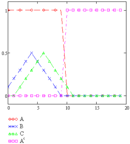
Example 4. Consider the fuzzy sets A , B , C and the complement A c with membership functions as shown in Figure 1. Note, that A and its complement are crisp sets. The distance matrix D = [ d i,j ] is shown in (8); the rows and columns correspond to A , B , C and A c so that for instance the element d 2 , 3 = dist ( B,C ) = 0 . 709 . As can be seen, C is a translated version of B and they are both the same distance from A . This is due to H ( X A glyph[triangle] B ( x )) = H ( X A glyph[triangle] C ( x +10)) . B and C are farther apart than B and A . Since dist ( A,A c ) = 0 then each one of B , C is of the same distance to A as to A c .

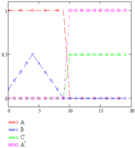
Example 5. Continuing with the same domain as in Example 4 let us consider the fuzzy sets A , B , C and the complement A c with membership functions as shown in Figure 2. The membership function of the set C is now flat and as the distance matrix D = [ d i,j ] in (9) shows C is now farther from B (which has a triangular membership function). As in the previous example B remains closer to A than to C .

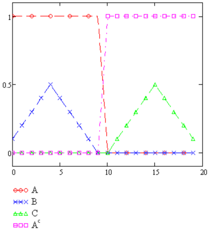
Example 6. Continuing with the same domain as in Example 4 let us consider the fuzzy sets A , B , C and the complement A c with membership functions as shown in Figure 3. Note that now C is translated from B by an amount that is smaller compared to Example 4. As can be seen from the distance matrix of (10) this results in a smaller distance dist ( B,C ) = 0 . 336 compared to 0 . 709 . As in Example 4 , A is as similar to B as to C since the distance dist ( A,B ) = dist ( A,C ) = 0 . 354 .

5 Clustering using the distance

We tested the proposed distance function on real data. The data 1 consists of answers from a survey given to the general population of 28 European countries. There are ten questions in the survey where a valid answer is a number in the set { 1 , . . . , 10 } . The value 10 represents the most positive opinion and 1 the most pessimistic opinion (we denote the name of the attribute in parenthesis):

• trust in local parliament ( country_GOV )
• trust in local politicians ( politicians )
• trust in EU Parliament ( EU_GOV )
• trust in United Nations ( UN )
• trust in country's parliament ( country_GOV )
• how satisfied with life ( Life )
• how satisfied with the national government ( National_GOV )
• immigration is bad or good ( Immigration )
• the state of health services ( Health )
• how happy are you ( happy )

After normalizing each component we represent each country as a fuzzy set on a domain that consists of the ten attributes. Table 1 displays the membership functions for each of the countries. Each row in this table represents a membership function m i ( x ) of the fuzzy set C i of country i . Based on this information we compute the distance d ( C i , C j ) between every possible pair of countries C i , C j and obtain a distance matrix D = [ d i,j ] , d i,j := dist ( C i , C j ) . We use D as the newly transformed version of the original data (Table 1) and do data-clustering on it. The i th row of D is a feature vector representation of country i . We use the k -means clustering procedure.

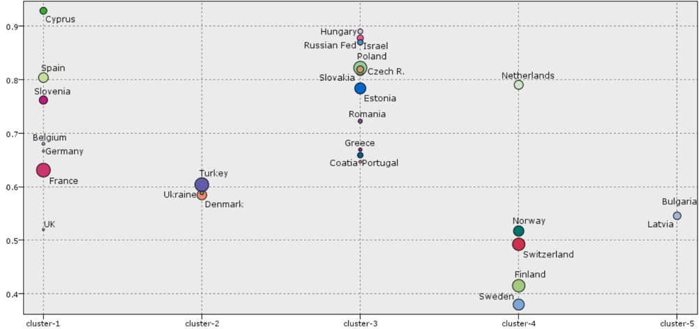
Figure 4 shows the result of the k -means clustering where the horizontal axis displays the cluster number and the vertical axis shows the distance of each point in a cluster to the mean of the cluster. In order to interpret this result, let us look at the fuzzy sets of some of the clusters. Figure 5 displays the fuzzy sets of cluster #1 . As seen, the country Spain is considered similar to the rest of the countries in this cluster although its 'happy' value is almost complement to the rest of the countries. This follows from the complement-property of our distance function (see section 4).

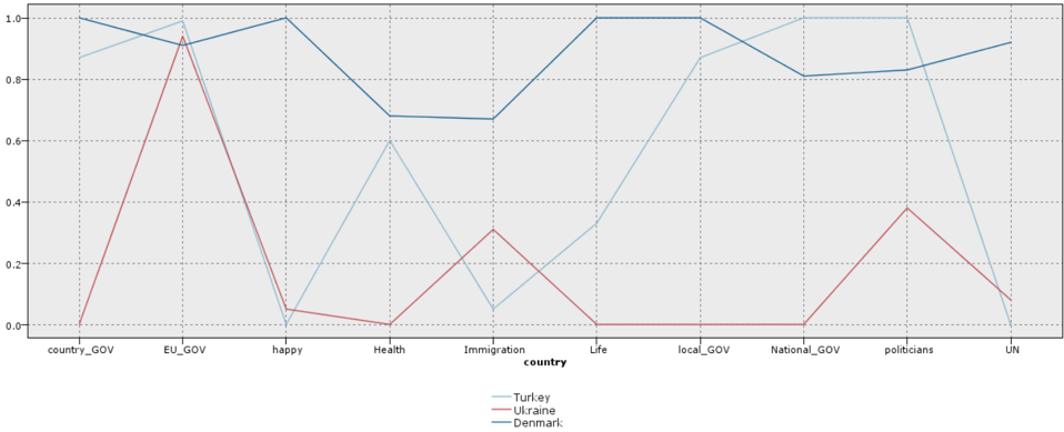
Figure 6 displays the fuzzy sets of cluster #2 . Ukraine seems to behave almost the opposite of Denmark (besides on the attributes EU_Gov where both have similar values). Ukraine and Turkey have interesting behaviors: they take very similar values for the attributes country-GOV up to Life and on UN while on the rest of the attributes they are almost mutually complement. Hence

1 The data set is the European Social Survey Round 4 Data (2008). Data file edition 3.0. Norwegian Social Science Data Services, Norway - Data Archive and distributor of ESS data. http://ess.nsd.uib.no/.

according to our distance they are considered close (which is why they are placed in the same cluster).

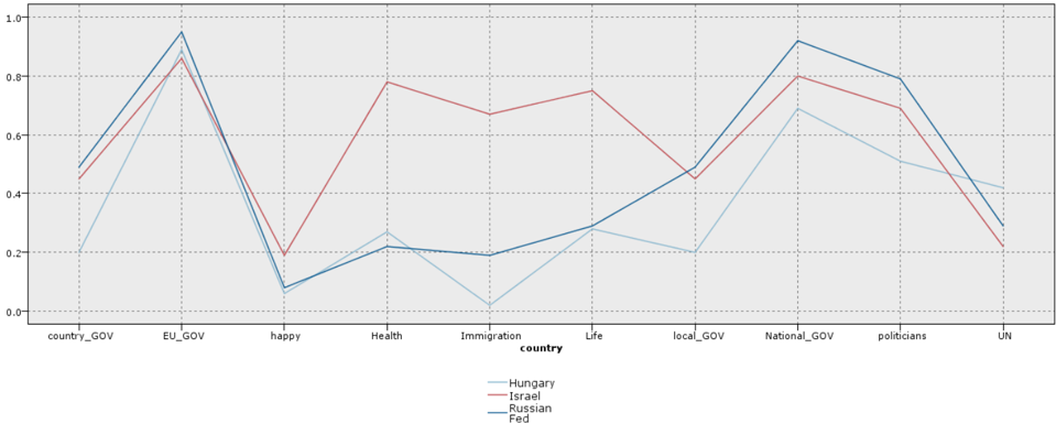
Figure 7 shows the fuzzy sets of several countries in custer #3 . Hungary and the Russian Federation take very similar values and hence are close. Israel versus Hungary or versus Russian Federation has a similar behavior on the attributes country_GOV , EU_GOV , happy , National_GOV , politicians , UN , while on Health , Immigration , Life it has almost the complement values. Hence, overall, our distance function renders Israel as close to Hungary and Russia.

We also ran a clustering procedure which is a variant of the Kohonen Self Organizing Map. The results that we obtained are very similar to those obtained by the k -means procedure.

6 Conclusion

This paper introduces a new distance function dist ( A,B ) for fuzzy sets A,B based on their descriptive complexity. The distance is shown to be a semimetric that satisfies the triangle inequality. In comparison to other existing distance-functions for fuzzy sets this new metric is proportional to the additional amount of information needed to describe fuzzy set A when knowing fuzzy set B or vice versa. It thus has a natural information-based interpretation. Doing pattern clustering based on this distance we have shown that fuzzy sets that are clustered together tend to be more mutually informative. This is an interesting new property that can be useful for analyzing other data sets.

References

1. R. Baeza-Yates and B. Ribeiro-Neto. Modern Information Retrieval . Addison-Wesley, 1999.
2. P. P. Bonisson. A pattern recognition approach to the problem of linguistic approximation in system analysis. In Proceeding of the International Conference on Cybernetics and Society , pages 793-798, 1979.
3. T. M. Cover and J. A. Thomas. Elements of information theory . WileyInterscience, New York, NY, USA, 2006. ISBN 0-471-24195-9.
4. M. Deza and E. Deza. Encyclopedia of Distances , volume 15 of Series in Computer Science . Springer-Verlag, 2009. ISBN 978-3-642-00233-5.
5. J. Ratsaby. Information efficiency. In Proc. of 33rd Conference on Current Trends in Theory and Practice of Computer Science (SOFSEM '07) , volume LNCS 4362, pages 475-487, 2007.
6. J. Ratsaby. Information width. Technical Report # arXiv:0801.4790v2 , 2008.
7. J. Ratsaby. Information set distance. In Proc. of Mini-Conference on Applied Theoretical Computer Science (MATCOS-10) , Koper, Slovenia, Oct. 13-14. University of Primorska press, 2010.
8. L.A. Zadeh. Fuzzy sets. Information Control , 8:338-353, 1965.

[9] R. Zwick, E. Carlstein, and D.V. Budescu. Measures of similarity among fuzzy concepts: A comparative analysis. International Journal of Approximate Reasoning , 1:221-242, 1987.

Figures and Tables

Belgium	0.60	0.55	0.69	0.60	0.60	0.72	0.47	0.48	1.00	0.30
Bulgaria	0.06	0.41	0.99	0.45	0.06	0.06	0.59	0.61	0.15	0.04
Switzerland	0.85	0.63	0.66	0.65	0.85	0.86	0.79	1.00	0.90	0.49
Cyprus	0.78	0.79	0.96	0.43	0.78	0.66	0.91	0.37	0.67	0.37
Czech R.	0.32	0.63	0.68	0.47	0.32	0.56	0.69	0.24	0.59	0.26
Germany	0.60	0.65	0.86	0.52	0.60	0.62	0.74	0.61	0.45	0.17
Denmark	1.00	0.83	0.91	0.92	1.00	1.00	0.81	0.67	0.68	1.00
Estonia	0.46	0.41	0.91	0.60	0.46	0.48	0.84	0.37	0.53	0.23
Spain	0.68	0.51	0.74	0.52	0.68	0.72	0.70	0.61	0.73	0.94
Finland	0.89	0.65	0.66	0.96	0.89	0.87	0.74	0.73	0.85	0.42
France	0.58	0.39	0.72	0.57	0.58	0.49	0.59	0.50	0.71	0.25
UK	0.54	0.62	0.53	0.52	0.54	0.66	0.75	0.39	0.71	0.28
Greece	0.40	0.49	0.87	0.26	0.40	0.43	0.69	0.00	0.17	0.15
Coatia	0.28	0.51	0.84	0.26	0.28	0.53	0.68	0.29	0.40	0.12
Hungary	0.20	0.51	0.89	0.42	0.20	0.28	0.69	0.02	0.27	0.06
Israel	0.45	0.69	0.86	0.22	0.45	0.75	0.80	0.67	0.78	0.19
Latvia	0.07	0.19	0.75	0.40	0.07	0.41	0.28	0.20	0.22	0.12
Netherlands	0.79	0.40	0.00	0.67	0.79	0.80	0.65	0.68	0.75	0.57
Norway	0.85	0.64	0.75	1.00	0.85	0.86	0.72	0.83	0.72	0.93
Poland	0.28	0.00	0.77	0.56	0.28	0.63	0.60	0.74	0.27	0.15
Portugal	0.39	0.51	0.81	0.50	0.39	0.34	0.72	0.58	0.38	0.16
Romania	0.45	0.75	1.00	0.67	0.45	0.44	0.77	0.66	0.30	0.08
Russian Fed	0.49	0.79	0.95	0.29	0.49	0.29	0.92	0.19	0.22	0.08
Sweden	0.84	0.70	0.64	0.90	0.84	0.85	0.75	0.73	0.73	0.47
Slovenia	0.57	0.74	0.92	0.51	0.57	0.64	0.90	0.33	0.48	0.24
Slovakia	0.52	0.69	0.95	0.61	0.52	0.52	0.84	0.30	0.38	0.19
Turkey	0.87	1.00	0.99	0.00	0.87	0.33	1.00	0.05	0.60	0.00
Ukraine	0.00	0.38	0.94	0.08	0.00	0.00	0.00	0.31	0.00	0.05

Table 1: Fuzzy membership values