Efficient enumeration of instantiations in Bayesian networks

Sampath Srinivas Microsoft Corporation One Microsoft Way Redmond, WA 98052 sampaths@microsoft. com

Abstract

Over the past several years Bayesian net­ works have been applied to a wide variety of problems. A central problem in applying Bayesian networks is that of finding one or more of the most probable instantiations of a network. In this paper we develop an efficient algorithm that incrementally enumerates the instantiations of a Bayesian network in de­ creasing order of probability. Such enumer­ ation algorithms are applicable in a variety of applications ranging from medical expert systems to model-based diagnosis. Funda­ mentally, our algorithm is simply performing a lazy enumeration of the sorted list of all instantiations of the network. This insight leads to a very concise algorithm statement which is both easily understood and imple­ mented. We show that for singly connected networks, our algorithm generates the next instantiation in time polynomial in the size of the network. The algorithm extends to arbi­ trary Bayesian networks using standard con­ ditioning techniques. We empirically evalu­ ate the enumeration algorithm and demon­ strate its practicality.

1 INTRODUCTION

Over the last several years Bayesian networks have been applied to a wide variety of problems rang­ ing from medical diagnosis [Heckerman et al., 1992; Horvitz et al., 1988] and natural language understand­ ing [Charniak and Goldman, 1991] to vision [Levitt et al., 1989] and map learnin g [Dean, 1990]. A c e n t ra l problem in such applications is to use the network to generate explanations for observed data. Such expla­ nations correspond to instantiations of the network (i.e., value assignments to each node in the network)

Pandurang Nayak Recom Technologies NASA Ames Research Center, MS 269-2 Moffett Field, CA 94035 nayak@ptolemy. arc. nasa. gov with the structure of the network providing the ex­ planation for the values. Each such instantiation has an associated probability that can be computed from the specification of the Bayesian network (see [Pearl, 1 9 88 a] for details). Hence, finding one or more of the most probable instantiations of a Bayesian network is a problem of central importance.

Pearl [1987] has developed an elegant message-passing algorithm for computing the most probable instanti­ ation of a Bayesian network. This algorithm runs in polynomial time on singly connected networks, and can be extended to arbitrary networks through con­ ditioning. It can also be used to compute the second most probable instantiation. Dawid [1992] has also developed an algorithm that computes the most likely instantiation using the junction tree of the Bayesian network. This algorithm is inherently applicable to arbitrary networks.

While generating the most probable instantiation is important, it is inadequate for a variety of applica­ tions. Instead, such applications require that differ­ ent instantiations of the network be enumerated in de­ creasing order of probability. For example, in a medi­ cal diagnosis application, the most probable diagnosis is rarely adequate; doctor's typically want the differen­ tial diagnosis, i.e., the set of plausible diagnoses that can explain the observed symptoms. The differential diagnosis is used in two ways: (a) to decide upon a set of tests that best distinguish between the various diagnoses; and (b) to help design a treatment plan, e.g., to select a plan that as applicable to all (or most) of the possible diagnoses. In Bayesian network terms, each diagnosis corresponds to an instantiation a n d a differential diagnosis is generated by enumerating in­ stantiations in decreasing order of probability.

Turning to another field, Hidden Markov Models (HMMs) have been used to find the most likely la­ beling of words with parts of speech in natural lan­ guage applications. The standard HMM model used in this application [Charniak et al., 1993] can be repre-

sented as a singly connected Bayesian network. Each labeling of words with parts of speech corresponds to an instantiation of the network. Current techniques compute the most likely labeling, i. e., the most likely instance of the corresponding Bayesian network. How­ ever, it may be happen that the most likely labeling is rejected by the semantic analysis phase of the nat­ ural language system. In such a situation, the next most likely labeling is necessary. Enumerating label­ ings in decreasing order of probability corresponds di­ rectly to the problem of enumerating instantiations of the Bayesian network in decreasing order of probabil­ ity.

Finally, enumerating instantiations of Bayesian net­ works is also needed to extend model-based diagnosis to handle dependent component failures. Some of the best model-based diagnosis algorithms [de Kleer and Williams, 1989; de Kleer, 1991] are based on enumer­ ating candidates in decreasing order of prior probabil­ ity, and checking these candidates for consistency with the observations.1 The enumeration algorithms used to date make the strong assumption that component failures are mutually independent. Dependent com­ ponent failures can be represented using a Bayesian network i!). which the nodes represent components and node values represent component modes, so that net­ work instantiations correspond to candidates. Existing model-based diagnosis algorithms can therefore be ex­ tended to handle dependent component failures using an algorithm to generate network instantiations in de­ creasing order of probability (see [N a yak and Srinivas, 1995]).

In this paper we develop an efficient algorithm to enu­ merate instantiations of a Bayesian network in decreas­ ing order of probability. Our algorithm can be viewed as a generalization of Pearl's message passing algo­ rithm for generating the most probable instantiation. We develop our algorithm in two phases. In the first phase, described in Section 2, we develop an algorithm to generate the entire list of network instantiations, sorted in decreasing order of probability. Of course, generating the entire list of network instantiations is impractical since the number of instantiations is expo­ nential in the size of the network. Hence, in the second phase, described in Section 3, we show how the above algorithm is modified to incrementally compute one instantiation at a time in decreasing order of proba­ bility. We analyze the complexity of the incremental algorithm in Section 4, and show that for singly con­ nected networks the next instantiation can always be generated in time polynomial in the size of the net­ work. In Section 5 we consider extensions to multiply

1 A candidate is an assignment of nominal or failure modes to components.

connected networks and to evidence nodes. Section 6 discusses experimental results from our implementa­ tion of the algorithms and demonstrates its practical­ ity. Section 7 discussed related work. We conclude in Section 8 with a discussion of future work.

2 COMPUTING THE ENTIRE LIST OF INSTANTIATIONS

Pearl [1987] describes a message passing algorithm for computing the most likely instance of a singly con­ nected Bayesian network. Our enumeration algorithm is also a message passing algorithm, and can be viewed as a generalization of Pearl's algorithm. It operates as follows. An arbitrary node in the Bayesian network is chosen as the starting node. The starting node re­ quests all its neighbors for messages pertaining to the computation of a list of instances sorted in decreasing order of probability. These messages pertain to instan­ tiations of the part of the network reachable through the neighbor. When the starting node has received the messages it combines them appropriately and returns the entire list of instantiations of the Bayesian net­ work sorted in decreasing order of probability. When a neighbor is requested to give a message, it recur­ sively requests each of its neighbors (except for the original requesting node) for a message. It combines these messages appropriately and passes them on to the requesting node. As we will see, the independence properties of the singly connected network make such a message passing algorithm possible.

The description of the message passing algorithm thus reduces to the description of the operations at a sin­ gle node. The description explains what the messages are and how the messages coming from neighbors are combined and sent to the requesting node. As noted earlier, we start by describing how to compute the en­ tire list of instantiations in decreasing order of proba­ bility. In the next section we show how to modify this algorithm to make it compute one instance at a ti m e (on demand).

2.1 WHAT ARE THE MESSAGES?

We now define the messages sent between nodes. We start by defining some terminology. Consider two nodes A and B that are connected by an arc in a Bayesian network R. We use RAIIB to refer to the set of all the nodes in the subnetwork containing A when t h e arc connecting A and B is disconnected. Note that the arc between A and B can be in either direction.

Suppose that node X requests node Y for a message, and let Y be a parent of X. We will refer to the mes-

sage that Y sends X as 1r�-+ x. 2 The direction of the arrow in the subscript refers to the direction of the message (from Y to X) and not the direction of the arc in the Bayesian network. The superscript l (for "list") reminds us that the message is being used to compute the ordered list of all instances of the Bayesian net­ work.

1!"�---+X is a vector indexed by the states y of Y. The location 1r� -+X [Y = y] contains a l i s t of all i n s t a n t ia ­ tions i of the nodes in Rnx such that Y has state y in i. The list elements are arranged in decreasing or­ der of probability. The probability is stored with each list element. Since R is a singly connected network, the elements in RYIIX form a complete Bayesian net­ work in themselves. Hence it is possible to compute the probability of each instantiation of RY\Ix without regard to X or any node reachable through X.

Now consider the case where Y is a child o f the request­ ing node X in the Bayesian network. We will refer to the message that Y sends X as >.�---+xThe >.� .... x message is indexed by the states x of X. >.� .... x[X = x] contains a list of instantiations r of Rnx sorted by de­ creasing o r d e r of the probability P(Rnx = r\X = x ) . This is the conditional probability of the instance r given X is in state x. The probability is stored with each list element.

Note that observing the value of X makes the nodes in RYIIX independent of all nodes in Rxuv· Hence given a state x of X and an instantiation r of RYIIX, it is possible to compute the probability P(Rnx = riX = x ) locally within the subnetwork formed by the nodes in Ryux·

2.2 COMPUTING THE MESSAGES

Suppose that node X has requested node Y for a mes­ sage. We describe the computations that Y performs in computing the message.

Y first recursively asks for messages from all its neigh-

2We follow Pearl in choosing 7f and .>.. as the message names.

bars (except for X). After they are available it com­ putes the message meant for X. There are two cases: Y is either a parent or a child of X.

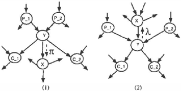
2.2.1 Y is a parent of X

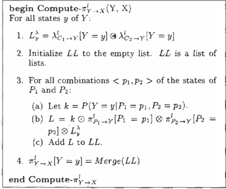
Consider an example of the first case (Figure 1.1). Say we are given an instance rp, I IY of the set RP,IIY, with H = P1 in r p1 1 J y. Similarly, say we are given an in­ stance rp2IIY of Rp2IIY· with P2 = P2 i n Tp2IIY· Fur­ thermore, let rc,IIY and rc211Y be any two instances of RcliiY and Rc2)IY·

If we append all these instances together and add in a choice of of state for Y, say Y = y, we get a full instance rnx of Rnx. The independence properties of a singly connected Bayesian network implies that:

Note that r Y IJX is an element of 7f�-+x[Y = y]. S i mi ­ larly r p11 1 y is an element of 7r�1-+ y [ H = p1] and r p211Y is an element of 1rh_.y[P2 = P2]· In addition, redlY is an element of .>.S1 .... y [ Y = y] and rc2uy is an element of Ab2 .... y[Y = y]. The probabilities required in Equa­ tion 1 are exactly those stored with these elements (see Section 2.1).

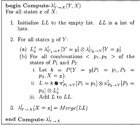
Figure 2 shows the algorithm that uses Equation 1 to compute the message 7r�_,x· The following terminol­ ogy is used in this algorithm. Given two,ordered lists of instances £1 and £2 ordered in decreasing order of probability, let £1 0 £2 be the ordered list composed of all possible combinations of the instances where one element is chosen from £1 and one element is chosen from L2. The probability of the combination is the product of the stored probabilities of the components. Given an ordered list of instances L and a number k, let k 0 L be the list where the probability of every instance in L is multiplied by k. Finally, given a list of ordered instance lists LL, let M erge(LL) be the list formed by merging the constituent lists of LL into a single ordered list. Each of the constituent lists of LL is assumed to contain instances of the same set of variables.

The discussion above leads directly to the algorithm in Figure 2. This algorithm computes 1!"� -+X from the messages coming to it from P1 , P2, C 1 and C2In essence, for each state y of Y, the algorithm is gen­ erating every element of n�_.x[Y = y] and ensuring that the elements are put together into a list in de­ creasing order of probability. The algorithm is easily

adapted to the case where Y has an arbitrary number of parents and an arbitrary n u m b e r of children.

2.2.2 Y is a child of X

Now consider the case where Y is a child of X. This situation is shown in Figure 1.2. The same argument used in the first case leads to the algorithm shown in Figure 3.3

3 At the expense of clarity, this algorithm can be im­ proved by computing and saving 1; for all y before enter­ ing the main loop.

2.3 COMBINING THE MESSAGES

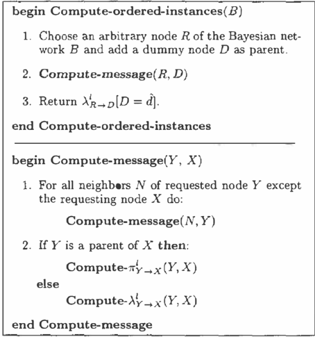
The algorithm Compute-ordered-instances for computing the ordered list of instances of the en­ tire Bayesian network follows directly from Compute­ 'll'� -+X and Compute->.� -+X.

We choose an arbitrary node R of the Bayesian net­ work as the root node and add a dummy node D as a parent of R. D has only one state d. Hence auto­ matically, P(D =d) = 1. Let the parents of R before adding D be the set SR. Let SR be a joint state of SR. Assume that the conditional probability was defined by the table Pozd(RISR)· The conditional probabil­ ity distribution of R after D's addition is set to be Pnew(R = riSR = SR, D = d) = Pald(R = riSR = sr). This ensures that effectively, R is independent of D, and hence if D requests R for a message, then .>.k-+d D = d] contains exactly the list of ordered in­ stances of the entire network. The full algorithm is described in Figure 4.

3 COMPUTING ONE INSTANCE AT A TIME

The previous section developed an algorithm that com­ putes the entire list of ordered instances. Hence, though it takes full advantage of the independence properties of the network to decompose the problem, it's run time is inherently exponential since the number

of instances is exponential. In this section, we modify that algorithm to return one instance at a time from the ordered list. The next instance is computed only on demand, i.e., we make the computation lazy.

Specifically, all that is required is to make the com­ putation of the list operations ®, 0 and Merge lazy. The modified Compute-ordered-instances returns a lazy list. Initially, a lazy list contains only the first element of the list. The rest of the elements are stored as a delayed computation in the list's data structure. Each time we demand the next element, the delayed computation is called. It performs only the necessary computations to compute the next element. This ele­ ment is added to the end of the list. The computation then delays itself again4.

Note that the list LL in Compute-trL_.x(Y, X) and Compute-,\�-+x(Y, X) is not a lazy list. However, each element in LL is a lazy list. This observation im­ plies that the delayed computations will perform only the list operations ®, 0 and Merge. Let the lazy ver­ sions of 0, @, and Merge be 0., ®z, and Mergez, respectively.

The definitions of 8z and M ergez is straightforward. Given a constant factor k and a lazy list Lz as argu­ ment 0z multiplies k into the probability of the first element of Lz and returns it. It then wakes up the delayed computation in Lz. This results in the second element of Lz being generated. It then goes to sleep. On the next call it multiplies the constant factor into the second element and returns it. It then generates the third element of Lz and goes to sleep and so on. On each call, it performs 0(1) computations (not counting the computation within Lz's delayed computation).

On each call, M ergez goes through its argument LL looking at the probability of the current element of every lazy list i n LL. It returns the element Cmax with maximum probability. Let Lmax be the list from which Cmax came. Cmax is popped off Lmax· Mergez now wakes up the computation of Lmax till the next element of Lmax is generated and this is made the current element of Lmax· It then goes to sleep. On each call, M ergez performs O(Length(LL)) compar­ isons (not counting the computation within the de­ layed computation of Lmax)·

3.1 AN EFFICIENT WAY OF MAKING ® LAZY

The operation @ takes two ordered lists L1 and LJ as arguments and returns an ordered list where e ach element is a compound element composed of one el-

4 See [ Charniak et al., 1987] for details on implementing lazy list operations.

ement from L1 and one element of LJ. The numeri­ cal value associated with the compound element is the product of the numerical values associated with the constituents. The list which is returned is ordered by this numerical value.

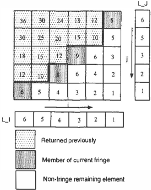
Consider the example shown in Figure 5. List L1 is shown along the rows of a matrix and list LJ is shown along the columns. In this example, the elements of the list are the numerical values themselves. Each lo­ cation in the matrix is the product of the appropriate elements of L 1 and L J.

An element a(i2,}2) in the matrix is dominated by an element a( i1, jt) if it is necessarily less than or equal to a(i1, h) regardless of the actual values in the or­ dered lists L1 and LJ. We see directly that a(i2,)2) is dominated by a(i1,j1) iff i1 :S i2 and ]I :S jz. We will call the element a(i + 1, j) as the dominated neigh­ bor along dimension i of a(i, j). That is, an element's dominated neighbor along a dimension is the element immediately "below" it along that dimension.

We will now describe 0z. Every time ®z is called, it returns the next largest element in the matrix. The remaining elements are those elements of the matrix that have not yet been returned during previous calls to 0 z. ® z encodes the set of remaining matrix ele­ ments using the fringe, F. The fringe consists of those remaining elements that are not dominated by any of the other remaining elements (see Figure 5).

Each time ®z is called, it returns the maximum el­ ement, Cmax, of the fringe F and then updates the fringe. The fringe update is easily accomplished by the procedure Update-fringe shown in Figure 6. Note that this procedure does not explicitly generate the

begin Update-fringe

1. Choose the max element Cmax of the fringe F and delete it from F.
2. Along each dimension K do: Cm.ax

Let CK be the dominated neighbor of along K. If C K is not dominated by any ele­ ment in F then:

• (a) Compute CK (i.e., actually multiple the probabilities and create the compound ele­ ment). This computation might require the computation of the next yet uncomputed element of L K. If so, awaken the computa­ tion of LK so that this element is available.
• (b) Add CK to the set F.
• Return Cmar.

end Update-fringe

Figure 6: Updating the fringe in IZlz·

matrix. It simply retains the matrix indices with each element of F to perform domination tests.

We have assumed in the above discussion that @z takes only two arguments. However, the identical discussion applies if there are n lists given as arguments. In­ stead of a two dimensional matrix, we have a n dimen­ sional matrix. The Update-fringe procedure applies even when there are n arguments. A general imple­ mentation that can handle any number of argument lists can be used to compute (L1 0z L21Zlz ... 0zLn) as IZlz(LI, L2, . · · , Ln)· Such an implementation is im­ mediately applicable in Compute-1r� -;.X (Y, X) and Compute-.X�_.x(Y, X).

Let Lresult be the entire ordered list which would result if all the elements returned successively by IZlz(LI, Lz, ... , Ln) were computed (by repeated calls to the delayed computation). Consider the situation where the first k elements of Lresult have been com­ puted and the rest are yet uncomputed. We see that every time we update the fringe, we add at most n ele­ ments to it. At the start of the computation the fringe consists of exactly 1 element (viz, the first element of Lresult). Hence after k elements of Lresult have been computed, the size of the fringe is at most nk. Examin­ ing Update-fringe, we see that when computing the k +1st element, we need O(nk) comparisons to deter­ mine Cmax· In addition, we need to make O(nk) dom­ ination tests along each of then dimensions in Step 2. Each domination tests requires n index comparisons. Hence the k + 1st element element of Lresult can be computed with O(n3k) comparisons (not counting any operations resulting from waking up computations in any argument list). We note that this is a loose bound.

In practice, as we shall see later, 02 does much better.

4 COMPLEXITY OF THE FULL LAZY ALGORITHM

We now compute an upper bound on the complexity of the full lazy algorithm, i.e., the complexity of gener­ ating the kth most probable instance of the Bayesian network.

Consider a node Y which is computing a message to be sent to node X u s i ng Compute-message(Y, X). Let Size(Y) be the size of the conditional probability table of Y. That is, Y is the product of the cardinalities of Y and each of its parents. Let Degree(Y) be the number of neighbors of Y, i.e., the sum of the number of parents and number of children.

We examine the complexity of computing the message where each message element is a lazy list. Specifi­ cally, we look at the total complexity of computing the next element in each of these lazy lists. We consider only the computations performed within Y, i.e., we exclude the comparisons performed in recursive calls to Compute-message.

Examining Compute-1r� -;.X (Y, X) and Compute­ >.� -;.X (Y, X), we ncte that the M ergez and 8z op­ erations together perform 0( Size(Y)) operations. 5

Now consider the number of operations performed by the ®z. Say we have generated the first k elements of every message element list and are looking to generate the k + 1st element of each of these lists. We see that the number of operations performed by ®z is bounded by O(Size(Y)Degree(Y)3k).

Given a Bayesian network B let Size(B) I:YEBSize(Y). We see that Size(B) measures the amount of information required to specify the network. Let MaxDegree(B) = maxYEBDegree(Y).

Say we have generated the k most probable instances of the Bayesian network and are now computing the k + lth most probable instance. We see that Gz and Mergez together perform O(Size(B)) operations. ®z performs 0( Size( B) M axDegree(B)3 k ) operations.

Thus, the overall complexity of generating the k + 1st most p rob a b le instance is 0( Size(B) M axDegree(B)3 k ) . Note that this is a loose upper bound. There are two reasons. The first is that the bound that we computed earlier on ®z is loose. The second is that we are assuming that every delayed list will be forced to compute its next element in the pro­ cess of computing the next most probable instance of

5In this analysis, we consider both comparisons and multiplications as elementary operations.

Table 1: Run times for Compute-orderedinstances.

Time to generate next instance
Number of Bayes net variables	300
Max. numb. of states per node	5
MaxDegree	5
Number of instances generated	600
Setup time	11 sees
Max. time	34 msec
Min. time	0 msec
Avg. time	7.8 msec

Time to generate next instance
Number of Bayes net variables	500
Max. numb. of states per node	6
MaxDegree	6
Number of instances generated	600
Setup time	2 mins
Max. time	50 msec
Min. time	0 msec
Avg. time	11.00 msec

the entire network. This need not be true. In practice, the algorithm runs much faster (as described later).

We also note that when k = 1 the algorithm computes the most probable instance of the network. This is exactly what is computed by [Pearl, 1987].

5 MULTIPLY-CONNECTED NETWORKS AND EVIDENCE NODES

The algorithm we have presented so far can han­ dle only singly connected Bayesian networks. When Bayesian networks are not singly connected, there is a general scheme called conditioning which can be used to adapt the singly connected algorithms to perform Bayesian network computations [Pearl, 1988b].

Conditioning chooses a set of nodes in the Bayesian network such that observing the values of nodes leaves the resulting network singly connected. This is in ac­ cordance with the independence semantics of Bayesian networks. The set of conditioning variables is called the cutset. A computation is performed for every possible joint instance of the cutset using the singly connected algorithm and these computations are then combined. In general, domains suitable for modeling with Bayesian networks have a large number of inde­ pendences and so the size of the cutset is small.

Our algorithm can be adapted directly to handle mul­ tiply connected networks using conditioning. For every joint instance c of the cutset, we compute an ordered list of instances Lc of the network. Each element ec of Lc will be a full network instance. Each element ec will necessarily have each of the conditioning variables in the state specified by c. The probability stored with ec will be P(eclc). Lc can be computed with the al­ gorithm we have developed above. For each list Lc we then compute L� = P(c) 8 LcHere P(c) is the prior probability of the cutset instance c. The lists L� (one for each cutset instance c) are then merged to give the list of all instances in decreasing order of probability.

Let the cutset of Bayesian network B be CB. Let Size(CB) be the size of the joint state space of the variables in the cutset. A loose up­ per bound for generating the k + 1st most prob­ able instance of the Bayesian network is then O(Size(CB)Size(B)M axDegree(B)3k). Thus, the k+ 1st most probable instance can be generated in lin­ ear time. We note however, that the problem of com­ puting the most likely instance of a Bayesian network, in general, is NP hard. In other words, the constant factor of our linear time algorithm can be extremely large (since it depends on the network characteristics). Thus, our enumeration algorithm is practical only for sparsely connected networks, i.e., networks for which O(Size(CB)) is small.

Finally, note that for simplicity of exposition, our al­ gorithm description has not made any reference to ev­ idence nodes. A very simple change makes the algo­ rithm generate only those instances which are consis­ tent with the evidence. These instances are generated in decreasing order of conditional probability given the evidence. The change is as follows: For each evidence node in the belief network, delete all states except the observed evidence state. Note that the probabil­ ities associated with the generated instances will be prior probabilities (i.e., without conditioning on the evidence). However, the posterior probability and the prior probability of each of the the instances is re­ lated by the same constant, viz, the prior probability of the evidence. Hence the instances are generated in the correct order (i.e., in decreasing order of posterior probability given the evidence).

6 IMPLEMENTATION RESULTS

The algorithm described in this paper has been im­ plemented in Lisp. The results reported below are for unoptimized compiled code in Allegro Common Lisp on a Sun Sparcstation 10. The run times reported are milliseconds of CPU time usage.

Run times for Compute-ordered-messages are shown in Table 1. The algorithm is implemented on top of IDEAL, a software package for Bayesian net­ work inference [Srinivas and Breese, 1990]. The times shown are for two randomly generated singly con­ nected belief networks. Given the number of nodes

n, we generated a singly connected Bayesian network nodes with n nodes. The maximum number of neigh­ bors for any node in the network (i.e., theM axDegree of the network) and the maximum nu m b e r of states for each node are also specified before the random Bayesian network is generated. The distribution for the belief network is set randomly.

We see that we can compute each instance in the order of tens of milliseconds on the average when the number of nodes is in the order of hundreds. The time to com­ pute instances varies fairly uniformly as the instances are generated. In other words, there is no trend to­ wards increase or decrease in the average time as the number of instances generated increases. We note here that if the algorithm performed in accordance with its worst case analysis there should be a linear increase in run time. In practice, we see that the algorithm does much better.

We note that the time to initialize the algorithm data structures is substantial relative to the time generate instances. Note that the initialization is a one time cost and can be incurred during off-line precomputa­ tion.

7 RELATED WORK

In addition to its use in explanation, the computa­ tion of most likely instantiations of Bayesian networks has been utilized in Bayesian network inference. [San­ tos and Shimony, 1994] approach the problem of com­ puting marginal probabilities in Bayesian networks by computing the most likely instances which subsume a particular state of a variable and summing over the probability masses of these instances. They formulate the problem of computing the most likely instance as a best first search and also as an integer programming problem. [Poole, 1993] searches through network in­ stantiations to compute prior and posterior probabili­ ties in Bayesian networks. A heuristic search function is used. In the model-based diagnosis community, [de Kleer, 1991] studies a closely related problem viz, how to focus the diagnostic search on most likely can­ didates. The common thread in the work discussed above is a best first search through the space of net­ work instantiations - in this paper, we have used the properties of Bayesian networks to reduce the search problem to a direct polynomial algorithm that per­ forms no search.

The work described in this paper is most closely re­ lated to the the results presented in [Sy, 1992] and [Li and D'Ambrosio, 1993]. In [Sy, 1992], the author sets up a search for finding the most probable explana­ tion with a particular pruning strategy. The pruning strategy is analyzed and found to yield a polynomial complexity bound for generating the next most prob­ able instance. [Li and D'Ambrosio, 1993] develop an algorithm to compute the next most likely instance by incrementally modifying "evaluation trees" of proba­ bility terms. Their algorithm too has a polynomial bound. Our algorithm's complexity is similar to that of [Sy, 1992] and [Li and D'Ambrosio, 1993]. However, in addition, it gives the additional insight that the un­ derlying operation is simply a lazy enumeration of the sorted list of all instantiations. This insight leads to a very concise algorithm statement which is both easily understood and implemented.

8 CONCLUSION

We have developed an efficient algorithm to enumerate the instantiations of a Bayesian network in decreasing order of probability. For singly connected networks the algorithm runs in time polynomial in the size of the network. An implementation of the algorithm re­ vealed excellent performance in practice. The algo­ rithm has significant applications including explana­ tion in Bayesian network-based expert systems, part­ of-speech tagging in natural language systems, and candidate generation (i.e., computing plausible hy­ potheses) in model-based diagnosis.

As described earlier, our algorithm can be used in model-based diagnosis to generate candidate diagnoses in decreasing order of probability (even when com­ ponent failures are dependent). The generated can­ didates are then checked for consistency with obser­ vations of the system. We plan to explore a tighter integration of candidate generation and consistency c h ec ki n g. The basic intuition is as follows: When a candidate is found to be inconsistent this gives us in­ formation that may allow us infer that some other can­ didates (which have not yet been generated) are nec­ essarily inconsistent. If this information is fed back to the candidate generator in some way, it can skip enumeration of such candidates. Such pruning has the potential to dramatically improve the overall efficiency of the diagnosis system.

One special case of interest is the situation where the component failures are independent i.e., a trivial Bayesian network with no arcs. The problem thus re­ duces to the following: Given a set of discrete variables X1, X2, ... , Xn and distributions P(Xi), successively compute joint instances in decreasing order of proba­ bility. We have developed a linear time algorithm for this special case - each successive instance is com­ puted in O(n). For this special case, we have also developed a tight integration between the candidate generation and consistency checking (along the lines described above). The result is a highly efficient and

focused search strategy [Nayak and Srinivas, 1995 ] .

We also plan to explore another very significant ap­ plication of our algorithm � viz, enumeration of most likely solutions in Constraint Satisfaction Problems.

Acknowledgements

We would like to thank the anonymous referees for their feedback and for pointers to some related work.

References

[Charniak and Goldman, 1991 ] E. Charniak and R. Goldman. A probabilistic model of plan recog­ nition. In Proceedings of AAAI-91, pages 160-165, 1991.

[Charniak et al., 1987 ] E. Charniak, C. K. Riesbeck, D. V. McDermott, and J. R. Meehan. Artificial In­ telligence Programming. Lawrence Erlbaum Asso­ ciates, Inc., Hillsdale, NJ, 1987.

• [Charniak et al. , 1993 ] E. Charniak, C. Hendrickson, N. Jacobson, and M. Perkowitz. Equations for part­ of-speech tagging. In Proceedings of AAAI-93, 1993.
• [Dawid, 1992 ] A. P. Dawid. Applications of a general propagation algorithm for probabilistic expert sys­ tems. Statistics and Computing, 2:25-36, 1992.
• [de Kleer and Williams, 1989 ] J. de Kleer and B. C. Williams. Diagnosis with behavioral modes. In Proceedings of IJCAI-89, pages 1324-1330, 1989. Reprinted in [Hamscher et al., 1992 ] .
• [de Kleer, 1991 ] J. de Kleer. Focusing on probable di­ agnoses. In Proceedings of AAAI-91, pages 842-848, 1991. Reprinted in [Hamscher et al., 1992 ] .
• [Dean, 1990 ] T. Dean. Coping with uncertainty in a control system for navigation and exploration. In Proceedings of AAAI-90, pages 1010-1015, 1990.
• [Hamscher et al., 1992 ] W. Hamscher, L. Console, and J. de Kleer. Readings in Model-Based Diag­ nosis. Morgan Kaufmann, San Mateo, CA, 1992.
• [Heckerman et al., 1992 ] D. Heckerman, E. Horvitz, and B. Nathwani. Toward normative expert sys­ tems: Part I. The Pathfinder project. Methods of information in medicine, 31:90-105, 1992.
• [Horvitz et al., 1988 ] E.J. Horvitz, J .S. Breese, and M. Henrion. Decision theory in expert systems and artificial intelligence. International Journal of Ap­ proximate Reasoning, 2:247-302, 1988.
• [Levitt et al., 1989 ] T. Levitt, J. Mullin, and T. Bin­ ford. Model-based influence diagrams for machine vision. In Proceedings of CUAI-89, pages 233-244, 1989.
• [Li and D'Ambrosio, 1993 ] Z. Li and B. D'Ambrosio. An efficient approach for finding the MPE in belief networks. In Proceedings of CUAI-93, pages 342349, 1993.

[Nayak and Srinivas, 1995 ] P. P. Nayak and S. Srini­ vas. Algorithms for candidate generation and fast model-based diagnosis. Technical report, NASA Ames Research Center, 1995.

• [Pearl, 1987 ] J. PearL Distributed revision of compos­ ite beliefs. Artificial Intelligence, 33:173-215, 1987.
• [Pearl, 1988a ] J. Pearl. Probabilistic Reasoning in In­ telligent Systems: Networks of Plausible In ference. Morgan Kaufmann, San Mateo, CA, 1988.
• [Pearl, 1988b ] J. Pearl. Probabilistic Reasoning in In­ telligent Systems: Networks of Plausible Inference. Morgan Kaufmann, San Mateo, Calif., 1988.
• [Poole, 1993 ] D. Poole. The use of conflicts in search­ ing Bayesian networks. In Proceedings of CUAI-93, pages 359-367, 1993.
• [Santos and Shimony, 1994 ] E. Santos and S. E. Shi­ mony. Belief updating by enumerating high­ probability independence-based assignments. In Proceedings of CUAI-94, pages 506-513, 1994.
• [Srinivas and Breese, 1990 ] S. Srinivas and J. Breese. Ideal: A software package for analysis of influence diagrams. In Proceedings of CUAI-90, pages 212219, 1990.
• [Sy, 1992 ] B. Sy. Reasoning MPE to multiply con­ nected belief networks using message passing. In Proceedings of AAAI-92, pages 570-576, 1992.