Efficient Estimation of the Value of Information in Monte Carlo Models

Tom Chavez l,2 and Max Henrion l,3

1 RockweJI International Science Lab, 444 High St., Palo Alto, CA 94301

2 Department of Engineering-Economic Systems, Stanford University

3 The Institute for Decision Systems Research, Inc., 350 Cambridge Ave., #380, Palo Alto, CA 94306

Abstract The expected value of information (EVI) is the most powerful measure of sensitivity to uncer­ tainty in a decision model: it measures the potential of information to improve the decision, and hence measures the expected value of the outcome. Stan­ dard methods for computing EVI use discrete vari­ ables and are computationally intractable for models that contain more than a few variables. Monte Carlo simulation provides the basis for more tractable evaluation of large predictive models with continu­ ous and discrete variables, but so far computation of EVI in a Monte Carlo setting also has appeared impractical. We introduce an approximate approach based on preposterior analysis for estimating EVI in Monte Carlo models. Our method uses a linear approximation to the value function and multiple linear regression to estimate the linear model from the samples. The approach is efficient and practical for extremely large models. It allows easy estima­ tion of EVI for perfect or panial information on individual variables or on combinations of variables. We illustrate its implementation within Demos (a decision modeling s y stem) , and its application to a large model for crisis transponation planning.

1.0 EVI: What's so, and What's New

Any model is inevitably a simplification of reality, and most of its input quantities are invariably uncertain. Sensi­ tivity analysis identifies which sources of uncertainty in a model affect its outputs most significantly. In this way, it helps a decision maker focus attention on what assump­ tions really matter. It also helps a decision modeler to assign priorities to his efforts to improve, refine, or extend his model by identifying those variables for which it will be most valuable to find more complete data, to interview more knowledgeable experts, or to build more elaborate submodels.

The expected value of information (EVI) on a variable xi measures the expected increase in value y if we learn new information about xi and make a decision with higher­ expected value in light of that information. It is the most powerful method of sensitivity analysis because it ana­ lyzes a variable's importance in terms of the overall pre­ scription for action, and it expresses that importance in the utility or value units of the problem. Other methods, such as rank-order correlation, express importance in terms of the correlation between an uncertain variable and the out­ put of the decision model. There are many cases where a variable can show high sensitivity in this way, yet still have no effect on the selection of an optimal decision. Deterministic perturbation measures importance in utility or value units, but it ignores nonlinearities and interactions among variables, and also fails to measure a variable's importance in te rm s of that variable's ability to change the recommended decision.

One calculates EVPI (Expected Value of Perfect Infor· mation) in discrete models by rolling back the decision tree. The computation itself is straightforward in the sense that, to compute EVI, one simply places at the front of the tree the chance variables to be observed. The EVPI is computed as the difference between the expected value computed for this scenario and the expected value for the regular tree, without observations.

Computing EVI with continuous variables is less intuitive, because we have no tidy way of reversing the uncertainty, unlike the discrete case. Yet continuous models are increasingly the norm for risk and decision analysis, first because discretizing inherently continuous variables intro­ duces unnecessary approximation, and second because Monte Carlo methods and their variants (e.g., Latin hyper­ cube) generate tractable, highly efficient solutions to pre­ dictive models that contain thousands of variables. An especially useful feature of the Monte Carlo method is that, for a specified error, the computational complexity increases linearly in the number of uncertain variables [Morgan and Henrion, 1990]. Exact methods require com­ putation time that is exponential in the number of vari­ ables.

There is thus a need to develop flexible, efficient methods for computing EVI on continuous variables in a Monte Carlo setting. A ftexible method has (I) the ability to com­ pute EVI on single variables or on any combination of variables, and (2) the ability to compute both perfect and partial values of information. Perfect information removes uncertainty entirely. Partial information reduces uncertainty.

We present a general framework for calculating EVI based on preposterior analysis. Using that framework, we develop a technique for computing EVI that depends on a linear approximation to the value function and on multiple linear regression to estimate the constants for the linear function. We also discuss a heuristic method for measuring the value of partial information in terms of what we call the relative information multiple (RIM). We have implemented these methods in detachable computational modules using Demos, a decision modeling system from Lumina, Inc., Palo Alto, CA. We demonstrate their use on a large model to aid in military transportation crisis plan­ ning.

2.0 Framework

A decision model consists of a set of n state variables x1, ·· ,x n , which we will denote by X. The decision maker has control of a decision variable D, which can assume one of m possible values d1 , .. ,dm. The value or utility func­ tion v(X,di) expresses the payoff to the decision maker when X obtains and decision di is chosen.

In a typical decision model, the state variables are uncer­ tain. We express prior knowledge about X in the form of a probability distribution, denoted {XI �},where �denotes a prior state of information. The optimal Bayes' decision maximizing the expected value 1 is given by

The optimal decision given perfect information on state variable x , denoted d * _., is

We define EVPI on x as

In a similar fashion, we define the optimal expected­ value decision given the revelation of evidence e, d* e· as

2.1 Binary decisions and Function z

Let us consider a simplified decision problem with two decision alternatives: one of them is the optimal Bayes' decision d*; the other we denote tr".

In view of the uncertainty in the state variables, there must exist uncertainty in the outputs as well. Thus, for each

1. We use Howard's inferential notation (see, for example, Howard, 1970). {XIS) denotes the probability de n s i t y of X condi­ tional on S; (XIS) denotes the expectation of X co n d iti o n a l on S.

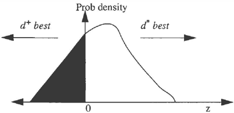
decision d;, there exists a unique probability distribution on value { v(X,d;)l �} (see Figure 1). For notational conve­ nience we let

We now define

Function z is the pivotal element in our framework for computing EVI because it describes the difference in value between the best and second-best decisions. In Figure 2, we have graphed the probability distribution of z. The shaded area represents the total probability of making a bad decision, i.e., doing d' when cY would yield higher value. Exploiting information encoded in the shaded, neg­ ative portion of the z distribution's curve will provide the necessary clues to compute EVPI and EVI.

In fact, we can use the intuition behind Figure 2 to write an expression for the general EVPI, which is EVPI on all state variables. The absolute value of z in the negative shaded portion is the utility that we could gain by chaos- ing cY instead of d'; its probability is just its correspond­ ing value on the density curve. Therefore, we have that

2.2 Preposterior Analysis

Preposterior analysis helps us to calculate the effect on X of our seeing evidence e, given a prior state of information �. At the heart of preposterior analysis is the specification of a preposterior distribution, which is a a prior proba­ bility distribution on a posterior mean. Probability theory provides a principled basis for calculating a preposterior distribution, given a prior and an adequate means of speci­ fying the effects of learning new information.

How do we represent perfect information on a continuous random variable X? If X were known with certainty, then its variance would be equal to 0. Thus, we can think of evi­ dence e as an information-gathering activity that somehow reduces the variance of X to 0. Evidence e that provides partial information reduces the variance on the prior of X, without shrinking that prior to 0.

The following lemma, taken from basic probability theory, is known as the conditional expectation formula.

A further useful result is the following lemma, which gives the formula for conditional variance.

Let J.l' and u' 2 z denote the prior mean and variance of z. They � e computed from our prior uncertainties X and our value function v. If we observe e, then we might ask how e influences z; in particular, we would like to know howe affects J.l' . We will denote the posterior mean of z given evidence � by J.l" .The distribution { J.l" I�} is a prior denz z sity on the posterior mean J.l" ; that is, it is a preposterior density. Substituting J.l" for t h e inner (XI e) on the right­ z hand side of the equation in Lemma 1 reveals that

Eq. 2shows that the mean of the preposterior distribution { ll" I � } is the same as the prior mean ll' . z z

If cr" 2 denotes the posterior variance of z after e, then z application of Lemma 2 shows that

If the prior and posterior on z are normal, then, as proved in [Raiffa and Schlaifer, 1961], the preposterior on z is normal also. That is, the normal distribution is conjugate to the normal sampling process. We thus require z to be distributed normally.

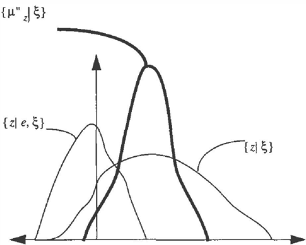
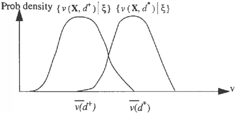
In Figure 3, we show a prior on z. a possible posterior on z given evidence e, and a preposterior density { ll" I� } . z Note that the preposterior has the same mean as the prior, and that its variance is the difference between the prior variance and the posterior variance.

The preposterior density encodes a state of knowledge about z in light of what evidence e might reveal. Its inter­ pretation is the same as in Figure 2. Because it is a proba­ bility density on value, we can integrate over its negative area to calculate the EVI of evidence e. Thus, we have

The type of integral given in Eq. 4 is known as a linear loss integral. In general, such an integral is impossible to evaluate analytically, so we must rely on statistical tables or numerical approximatation methods to evaluate it.

3.0 Complexity and Non-Additivity of EVI

Inference in probabilistic models with discrete variables is exponential in the number of vari a b l e s , so we would expect the exact calculation ofEVI to be exponential in the number of variables also. For simplicity, we assume a single decision variable with m alternatives. Let k; be the number of states for the ith state variable x;. To evaluate a decision tree with n state variables, we require a number of value computations at the leaves equal to

i= 1

Computing EVI on some subset of variables requires at least the same number of value computations at the leaves, and thus we see that exact calculation of EVI is e x pone n ­ tial inn. Also note that EVI calculations in discrete models are possible for perfect information only.

If c; represents the value of information on state variable X;, and C represents the value of information on all the state variables simultaneously, then

The above relation makes it difficult to devise separable, or incremental, procedures for computing EVI, because EVI will often demonstrate nonlinearities for varying combinations of variables and for varying cases of perfect and partial information.

4.0 Approximation of EVI

We are ready to apply the preceding analysis to develop an efficient algorithm for estimating EVI. We introduce a lin­ ear approximation to the value function, which in tum allows us to derive an expression for z, the net difference in value between two decision alternatives. Preposterior analysis on z provides a flexible mechanism for estimating EVI.

4.1 The Linear Value Model

We require a key approximating assumption: The value function v(X,d;) can be approximated by a first-order (linear) equation for each decision d;. that is, we can write v; as a linear function of the x; .

We assume, for now, that the x; are independent. (The assumption is not necessary; we use it to simplify our pre­ sentation.) We denote the prior mean of x; by �·; and denote its prior variance by cr'2;. Our approximating assumption allows us to perform simple but useful proba­ bilistic analysis. First, by linearity of expectation, we can write the mean ii (d ; ) as

Second, the variance of { v(X,d;)} can be written as

By our approximating assumption, we can write a linear approximation for v(X,d\

and one for v(X,d+),

Combining Eqs. 5-8 with the definition of z, we can write expressions for the prior mean and variance of z:

Suppose that e expresses perfect information on xk and no information about the other x ; . Let cr" i denote the poste- rior variance on xk. Since e is perfect information on x k , cr" �=0. Eq. 10 gives an approximation to the prior vari­ ance on z, cr';. Given e, we know that the kth term in the expression in Eq. 10 must be equal to zero. We can thus write the posterior variance for z given e, cr" 2: z

In view of Eq. 3, the preposterior variance on z is

4.2 Monte Carlo methods: Estimation of the Coefficients

In Monte Carlo simulation, we generate a sample of n sce­ narios by sampling from the prior distriubtions {XI�}. A scenario Xs is ann-tuple of state- variable assignments to X. v(Xs,di) is equal to the value or utility generated by the sth scenario for the ith decision alternative.

We can estimate the expected value of each decision d1 as the average of the values v(Xs,di) over the scenario i n d e x s. The optimal Bayes' decision is the maximum of those averages. (Naturally, higher sample sizes give answers of greater precision.) We represent this process for our binary decision problem in Table 1:

TABLE 1. Determining the optimal decision in Monte Carlo decision ar�alysis with sample size= 100 and two decision alternatives

sth Scenario	Value with d1	Value with d2
XI		v(X1,d2)
Xwo	v(X100,d1)	v (X 1ro d 2)
Average	100v(X d) L s' I 100 s =I	too v (Xs, d1) 2: 100 s=1

The o nl y outstanding task is to estimate the constants for the linear-approximation model. To this end, we apply multiple linear regression analysis to estimate the con­ stants in Eqs. 7 and 8. Let i b e an index into set of m deci­ sion alternatives, and letj be an index into th e n state variables. From [Shavelson, 1988], we can use mu l ti ple linear regression to write constants for v;value for the ith decision alternative in terms of the n state variables­ as follows:

where Rij = correlation(vi,x). Ru= correlation(xi,x ) ,S;= standard deviation(v;), and o ;=standard deviation(xj). We estimate these q uan t i ties directly from our Monte Carlo samples.

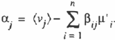
Recall from Section 2. 1 t ha t the v; generate probability distributions in a Monte Carlo model. Thus, it m a k e s sense to think of them as random variables with corresponding sample correlations and standard deviations. The a. are estimated as follows: 1

4.3 Relative Information Multiple

Suppose now that e expresses partial, rather than p er fe c t , information on xk. It is not immediately obvious how to specify partial information on an uncertain variable. We suggest the f o llo w in g method, based on our concept of a RIM. A RIM of evidence e on variable xk is defined to be the ratio between the p r i o r variance o ' i and the p os teri o r variance o " � on xk after e has been seen. In intuitive terms, the RIM measures how much we could know rela­ tive to what we know now. It is a m u lti pl e on missing but knowable information. For example, if an information source could tell me roughly twice as much as I know now, then the equivalent RIM is 2.

A var ia b l e xk's contribution to the prior variance o-' 2 is . . Eq 10 rt* + 2 2 z g 1ve n m . as (pk -� k) o ' k.For aRIM=rofevidence e on variable xk, the posterior variance o" 2 is given by z

The preposterior variance is es t i m a t e d as

The p r e p o st er i o r mean for partial information stays the same, as in Eq. 9.

4.4 Z Is Normal

We will assume that the x;, are normally distributed. In light of the following p ro po sit i o n from probability theory, our linear-approximating assumption requires z to be normally distributed also.

Proposition: Let X; be a collection of n normal random variables with means g i ve n by J..li and variances o 2 · Define the random va ri a bl e Y as '

Then Y is n o rm all y distributed also, with mean given by

and variance

0

Observe t h a t our approximating assumption allows us to write the mean and variance of z using standard probabil­ ity formulae. There is nothing about our framework, how­ ever, that forces the actual distribution of z to b el o ng to the same family as do z's component distributions. For exam-

ple, if the x; are Poisson, normal, and exponential, then z is a hard-to-assess, mongrel distribution. Assuming that the xi are normal forces z to be normal also. If the x; are non­ normal, then we must make an extra approximating assumption that z is normal also, although we must emphasize that this assumption would not be analytically true.

A limiting aspect of the technique presented here is that it measures EVI relative to only two decisions. In [Chavez, 1994], we show how to extend it to accommodate multiple (�3) decision alternatives.

4.5 Algorithm for EVI

We now summarize, in algorithmic form, our general tech­ nique for estimating EVI in a Monte Carlo decision model:

1. Select the two decision alternatives generatin ¥ the highest and second-highest expected value, d and cr.
2. Define variable z as the difference between v(X,d*) and v(X,d+).
3. Calculate regression constants � �, � +,a·, and a+. I I
4. Using Eqs. 2 a n d 9, calculate the mean (!l " zl s> of the preposterior distribution of z: ·

1. For perfect i n fo rma t i on on Xi, define

1. For partial information on Xi with RIM=k, define

1. For perfect information on variables with indices in S, define

1. F o r partial information on variables with indices i a nd a corresponding ordered set of RIM's k;, define

1. For perfect information on variables with indices in S mixed with partial information on variables with indi­ ces i and a corresponding ordered set of RIM's k;.

• 10.Define the preposterior density on z, {!l" z l S}, as

1. Express EVI as

1. Perform the integration in (11) numerically.

5.0 Application

We now describe an application of our method to a large decision model developed at Rockwell's Palo Alto Science Laboratory to support Course of Action (COA) analysis for Noncombatant Evacuation Operations (NEO). Implemented in Demos, NEO-COA allows a user to instantiate a generic NEO plan with specific parameter values for locations, forces, and destinations of troops and civilians. The model provides insights into the relative strengths of alternative plans by scoring them using differ­ ent evaluation metrics, such as time to complete the opera­ tion. Because many of the elements of a real-world military planning scenario are not known with certainty, several of the model's inputs are specified as continuous probability distributions.

In the current version of NEO-COA, there are three deci­ sion variables, or factors over which a military planner exercises control:

• Security forces: Security forces vary in their starting locations, dates of availability, and capabilities in pro­ viding security.
• Safe havens: The places where civilians gather to take shelter, safe havens differ in terms of distances from the assembly areas and port capacities.
• Transportation assets: A configuration of transporta­ tion assets is a sequencing of transportation capability over a fixed period of time. "Three C-141 's available

on day 2 and 5 C-14l's on days 3 through 10" is an example of a particular transportation configuration.

Because each of these decision variables currently possess three alternatives, there are a total of 27 available courses of action. In addition, the NEO-COA model possesses over 100 different input variables; of those, currently nine are specified as probabilistic quantities.

Once the decision variables and inputs have been speci­ fied, the model performs a dynamic simulation of the flow of U.S. citizens (the non-combatants) from their starting locations within a country to a set of selected assembly areas, and then on to the safe havens. It also includes risk factors associated with both U.S. citizens and U.S. mili­ tary personnel as functions of time. For example, risk to U.S. citizens at the assembly areas can rise and fall over the course of an entire operation in response to uncertain events, such as the arrival of security forces. The func­ tional representations of the risk factors are then used to compute expected casualties- civilian and military for varying alternatives.

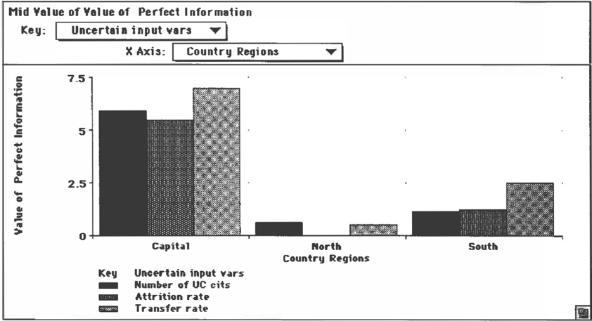
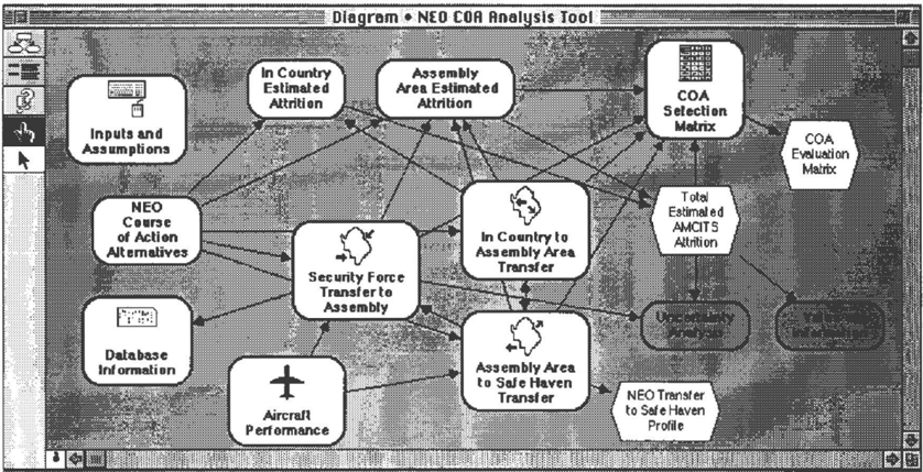
A top level view of the NEO-COA model as implemented in Demos is shown in Figure 4. There are three uncertain­ ties for the NEO-COA model: Initial USCITS, pr o b a bil ­ ity distributions on the number of U.S. citizens in each of the three regions of the country (capital, north, and south) at the start of a crisis planning operation; Country Regions Attrition Risk, which is the risk posed to non­ combatants over the course of an operation; and Transfer Rate, wh ic h is the speed at which civilians move from their starting locations to the assembly areas. Thus a total of nine continuous probability distributions must be assigned; typically, these are subjective assessments pro­ vided by military planners using the model.

In Figure 5, we show the results of applying the EVI approximation technique to the NEO model for perfect information. We see, for example, that the uncertainty about the number of American citizens in the capital has EVI equal to about six lives, and the uncertainty about the transfer rates in the capital has perfect information value equal to more than seven lives. In all cases, the value of information is highest for uncertainties relating to the cap­ ital region, reflecting that the highest number of citizens are concentrated there. The integral in Eq. 4 is evaluated numerically. Perfect information calculations on nine uncertainties took Demos 1 minute, 53 seconds running on a Macintosh Ilfx computer.

6.0 Conclusions and Future Directions

We have described a general analytic framework for esti­ mating EVI in a decision model using preposterior analy­ sis. It employs a linear-approximating assumption that allows us to write the value function as a first-order equa­ tion in the inputs. We define variable z to be the difference in value for the two decision alternatives. Multiple linear regression on the inputs provides the necessary constants for the linear value equation; we estimate the regression constants from Monte Carlo sample information. Applying preposterior analysis to z allows us to write an approxima­ tion to the value of perfect and partial information for any combination of state variables.

There are several areas in which we plan to extend the work presented here. First, we would like to develop a sis­ ter technique for approximating EVI on continuous deci­ sion variables. Second, we would like to examine how well our technique performs relative to an exact, more costly approach. To this end we will apply our method to several large models, run it several times, and compare its results to the corresponding exact answers. Third, we wilk apply statistical proof techniques to analyze formally the algorithm's convergence and error characteristics.

7.0 References

Chavez, Tom. (1994). "Recovering Value oflnformation from Pairwise Peeks," Rockwell Palo Alto Science Lab. Technical Memorandum.

Hennon. Max and Morgan, Granger. (1990). Uncertainty: A Guilk ro Dealing with Uncertainry in Quantitative Risk and Policy Analysis. Cambridge University Press. Cambridge.

Howard. R. A. (1970). "Proximal Decision Analysis." Management Science, 17, No. 9:507-541.

Raiffa, Howard and Schlaifer, Raben. (1961 ). Applied Statistical Decision Th�ory, MIT Press, Boston.

Shavelson, Richard. (1988). Statistical Reasoning for IM Behavioral Sciences. 2nd ed. A ll y n and Bacon, Inc, Boston.