Efficient Value of Information Computation

Ross D. Shachter

Engineering-Economic Systems and Operations Research Dept.

Stanford University Stanford, CA 94305-4023 [email protected]

Abstract

One of the most useful sensitivity analysis techniques of decision analysis is the com­ putation of value of information (or clair­ voyance), the difference in value obtained by changing the decisions by which some of the uncertainties are observed. In this paper, some simple but powerful extensions to pre­ vious algorithms are introduced which allow an efficient value of information calculation on the rooted cluster tree (or strong junction tree) used to solve the original decision prob­ lem.

Keywords: value of information, clairvoyance, clus­ ter trees, junction trees, decision analysis, influence diagrams.

1 Introduction

The analysis of sequential decision making under un­ certainty is closely related to the analysis of probabilis­ tic inference. In fact, much of the research into efficient methods for probabilistic inference in expert systems has been motivated by the fundamental normative ar­ guments of decision theory. Previous research has ap­ plied those developments by modifying algorithms for efficient probabilistic inference on belief networks to address decision making problems represented by in­ fluence diagrams (Jensen and others 1994; Ndilikilike­ sha 1991; Shachter and Ndilikilikesha 1993; Shachter and Peot 1992; Shenoy 1992).

One of the most useful sensitivity analysis techniques of decision analysis is the computation of value of in­ formation (or clairvoyance), the difference in value ob­ tained by changing the decisions by which some of the uncertainties are observed (Raiffa 1968). In this paper, some simple but powerful extensions to previous algo­ rithms are introduced which allow an efficient value of information calculation on the rooted cluster tree (or strong junction tree) used to solve the original decision problem.

Dittmer and Jensen(1997) proposed that multiple value of information calculations could all be per­ formed using the same tree. It is this idea that this paper builds on.

Section 2 presents a brief introduction of influence di­ agrams and Section 3 reviews the most efficient meth­ ods for solving them. Section 4 develops some new results which are in applied in Section 5 to efficiently perform multiple value of information calculations. Fi­ nally, Section 6 provides some suggestions for future research.

2 Influence Diagrams

Influence diagrams are graphical representations for decision problems under uncertainty. In this section the components and notation of influence diagrams are briefly introduced. The graphical structure of the in­ fluence diagram reveals conditional independence and the information available at the time decisions must be taken. This is a cursory introduction and the reader is referred to the relevant literature for more informa­ tion.

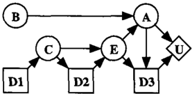
An influence diagram is a directed graph network rep­ resenting a single decision maker's beliefs and prefer­ ences about a sequence of decisions to be made un­ der uncertainty (Howard and Matheson 1984). The nodes in the influence diagram represent variables­ uncertainties (drawn as ovals), decisions (drawn as rectangles), and the criterion values for making deci­ sions (drawn as diamonds). The parents of uncertain­ ties and values condition their distributions, while the parents of decisions represent those variables that will be observed before the decision must be made. The value represents the expected utility of its parents, and decisions are made to maximize this expected utility. When there are multiple value nodes, the total utility is the sum of the utilities for each value. (The results in this paper could also be applied to products (Shachter and Peot 1992; Tatman and Shachter 1990).)

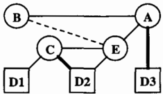
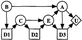
Consider the influence diagram shown in Figure 1 from Dittmer and Jensen(1997). There are four uncertain­ ties, A, B, C, and E, three decisions, D1, D2, and D3,

一

and a single value, U. The decisions are ordered in the graph and information available at the time of one decision is remembered for subsequent decisions, the no forgetting principle. For example, D1 and C are .ob­ served before both D2 and D3, while Dz, E, and A are observed before only D3. None of the variables are ob­ served before D1 is chosen. Not all of the observations are really needed or requisite for a decision. For exam­ ple, although five of the variables are observed before D3 is chosen, A is the only requisite observation-once A has been observed, the other variables provide no additional information. Similarly, C is the only requi­ site observation for Dz. The diagram can be analyzed to determine the maximal expected utility. If the util­ ity does not represent dollars, we could convert it to dollars by applying the inverse of the utility function that maps from dollars to utility.

We can solve a different decision problem without changing any of the distributions in the uncertainties and values by changing the informational assumptions. For example, in Figure 2 B is now observed before D1 is chosen. The expected utility from this diagram must be at least as much as from the earlier diagram because of this extra information, the opportunity to observe B. The influence diagram makes it explicit what information is available and when it is available in the two diagrams. This extra value leads to a differ­ ence in dollar values called the value of information or value of clairvoyance. Technically, the value of infor­ mation is only approximated by this difference (Raiffa 1968), but we will work with this approximated value. Without any new assessments, the decision problem can thus be solved many times, varying the informa­ tional assumptions for one variable at a time. This is the process this paper seeks to perform efficiently.

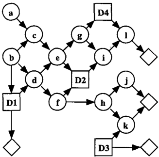
Another influence diagram example that will appear in this paper is shown in Figure 3 (Jensen and oth­ ers 1994). This diagram has four value nodes, whose

functions are summed to obtain the expected utility.

The influence diagram has been developed as a practi­ cal representation for a decision problem, and to that end there are several semantic restrictions, which are described in detail elsewhere (Howard and Matheson 1984; Shachter 1986). In particular, we cannot ob­ serve the descendant of a decision before making the decision, since the decision can affect its descendants. The one exception is when the descendant represents a constraint and is a deterministic function of the deci­ sion and its requisite observations. But this case could be modeled as a value node (with certain cases hav­ ing prohibitive value) instead of as an observation and thus we can exclude it without loss of generality.

3 Rooted Cluster Trees

Efficient algorithms have been developed to solve de­ cision problems represented as influence diagrams. These algorithms build an auxiliary structure called a rooted cluster tree or strong junction tree. Previous work has suggested how value of information calcula­ tions could be performed efficiently on such a tree.

Although the influence diagram can be solved directly (Shachter 1986), the most efficient procedures work on related graphical structures (Jensen and others 1994; Ndilikilikesha 1991; Shachter and Ndilikilikesha 1993; Shachter and Peat 1992; Shenoy 1992). This paper considers one of those graphical structures, the rooted cluster tree, a slight generalization of the strong junc­ tion tree.

A set of variables is called a cluster. A tree of clus­ ters is called a cluster tree (or join tree) if every de­ cision or uncertainty appears somewhere in the tree 1 ,

1 If the cluster tree were not being constructed to compute value of information, it might be worthwhile to exclude vari­ ables determined to be extraneous, but here it is desirable to keep all of the variables in the model.

each uncertainty and its parents appear together in at least one cluster, and any variable that appears in two different clusters appears in all of the clusters on the path between them. Corresponding to the notation in Jensen et al(1994), there are two potential functions associated with each cluster C, a probability poten­ tial, ¢c, and a utility potential, 1/Jc. This paper will introduce and present a minimal amount of this nota­ tion, instead focusing on other extensions to Jensen et al(1994). All of the tables in the influence diagram are incorporated into these potential functions.

The cluster tree is rooted if the arcs between clusters are directed so that one cluster, the root cluster, has no children, and all of the other clusters have exactly one child. It is useful to distinguish between clusters and variables by their location relative to the root. Cluster C is inward of another cluster C' in a rooted cluster tree if C is either the root cluster or between the root cluster and C'. In that case C' is said to be outward of C. If all clusters containing a variable A are outward of some cluster containing a variable B then A is strictly outward of B and B is strictly inward of A. If all clusters containing A either contain B or are outward of a cluster containing B, then A is weakly outward of B and B is weakly inward of A. For example in Figure 5, k is strictly outward of h, strictly inward of j, and neither weakly inward nor weakly outward of g.

There are other restrictions that have been developed for rooted cluster trees, but for simplicity only the fol­ lowing, new definition will be presented here. A rooted cluster tree is properly constructed for an influence di­ agram if

1. decision D is strictly inward of decision D' only if D must be chosen before D';
2. decision D is weakly inward of uncertainty A if A is a descendant of D in the influence diagram;
3. decision D is not strictly inward of uncertainty A if A will be observed before D is chosen;
4. decision D and its requisite observations are all contained in some cluster; and
5. any variable A strictly inward of decision D and also in a cluster with D is observed when D is chosen.

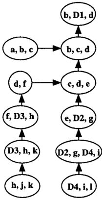
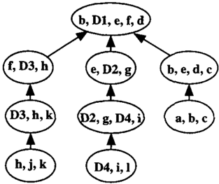
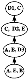
Rooted cluster trees properly constructed for the in­ fluence diagrams from Section 2 are shown in Figure 4 and Figure 5. The influence diagram's value can then be determined by making a single sweep through the rooted cluster tree toward the root, as summarized in Algorithm 1. The marginalization operator is de­ scribed in Jensen et al(1994).

Algorithm 1 (Value Calculation) This algorithm computes the optimal expected value on a properly con­ structed rooted cluster tree.

Visit each cluster C in the tree working inward from the leaves toward the root. That is, choose any cluster to visit whose outward neighbors have already been vis­ ited. When visiting a cluster, incorporate the updates from C 's outward neighbors, and marginalize all vari­ ables that do not appear in C's inward neighbor in an order consistent with observation.

At the end, the root cluster computes two scalar up­ dates, ¢0 representing the probability of the evidence and I/J0, where I/J0 / ¢0 is the expected utility of the op­ timal strategy. For value of information calculations, this latter quantity can be used directly or it can be converted to units of dollars {by applying the inverse utility function).

This algorithm is generalized in Dittmer and Jensen (1997) to perform multiple value of information calcu­ lations with only one cluster tree. The variable( s) to be observed earlier are added to inward clusters. For example, the tree in Figure 6 has uncertainty B added to the three clusters where it did not appear before.

It is not exactly clear how this expanded cluster tree should be processed. According to Dittmer and Jensen (1997), "As mentioned earlier, a control structure is associated with the (strong) junction tree. This struc­ ture handles the order of marginalization, and there­ fore we can use the expanded junction tree (and the associated control structure ) in Figure 7 c to marginal-

] 4

=

一

ize B from any clique of our choice. After B has been marginalized from a clique, the table space reserved for B in cliques closer to the strong root is obsolete. Clever use of the control structures will prevent calculations to take place in the remaining table expansions, and the number of table operations in the remaining sub­ tree equals that of an ordinary strong junction tree."

4 New Results

The definition for a properly constructed rooted clus­ ter tree introduced in Section 3 allows the derivation of some simple but powerful results that will be ap­ plied to perform value of information calculations in Section 5. But first it will be helpful to build the best possible rooted cluster trees for the original influence diagram.

The first step in building a cluster tree is recognizing which observations are requisite for the different de­ cisions. Although the BayesBall algorithm (Shachter 1998) is fast (linear time in the size of the graph), it is conservative in computing requisite observations, as­ suming that the value sets are nested. A less conserva­ tive algorithm can be fashioned by teaming BayesBall with the reductions in Tatman and Shachter(1990).

Algorithm 2 (Requisite Observations) This al­ gorithm determines the requisite obse1"'Uations for each decision in an influence diagram as a prelude to proper construction of a rooted cluster tree. It runs in time 0 ( (number of decisions) (graph size)).

Visit each decision Di in reverse chronological order, i = m, . . . , 1. Let v; be the set of value descendants of D in the current diagram. Run the BayesBall al­ gorithm on v; given Di and I;, the variables obse1"Ved before D; is chosen, and let fl. be the requisite obser­ vations (not including D;). Replace Di by a chance

node "policy" with R.; as parents and proceed to the next earlier decision.

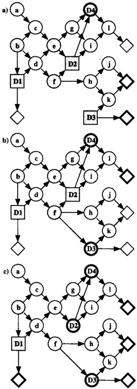
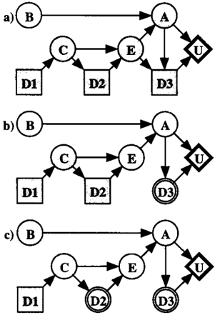
This algorithm is applied to the two influence diagrams from Section 2, as shown in Figure 7 and Figure 8. In the figures, the value descendants for a particular decision are highlighted, and the decision and its ob­ servations are shaded. In Figure 7, it can be seen that the requisite observations are R3 = {A}, R2 = {C}, and R1 = 0. In Figure 8, the requisite observations are R4 = {g, D2}, R3 = {!}, R2 = {e}, and R1 = {b}. Note the different sets of value descendants.

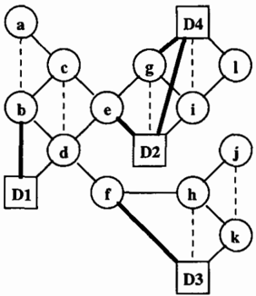
The next step is to generate the moral graph of the modified diagram. These moral graphs are shown in Figure 9 and Figure 10. The heavy shaded arcs cor­ respond to requisite observations, the dashed lines are moralizing arcs (added between parents with a child in common), and the value nodes have been removed (after any corresponding moralizing arcs were added).

Rooted cluster tree can now be properly constructed based on the moral graphs of the modified diagrams. There is no efficient algorithm to generate such trees, but the structure of the moral graph guides the process (Jensen and others 1994). It can be shown, however,

that the method just presented can always yield at least some properly constructed rooted cluster trees.

Theorem 1 (Requisite Observations) Al­ gorithm 2 can be applied to an influence diagram to yield a rooted cluster tree properly constructed for the diagram.

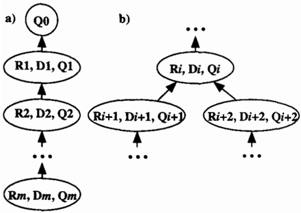
Proof: It is sufficient to show how one such rooted cluster tree could be properly constructed for any in­ fluence diagram. At each step of the algorithm, let Q be the non-value variables relevant to v; as deter­ mined by the BayesBall algorithm. (If we are building a rooted cluster tree for potential value of informa­ tion queries also add to Q any descendants of Di that could be observed. Otherwise, apparently extrane­ ous variables will not appear in the constructed tree.) Now let Q; be those nodes in Q for the first time, Q; = Q \ ( Q i+! U . . . U Qm)· Finally, let Qo be any nodes relevant to R1 that have not been included in QJ, ... ,Qm.

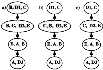
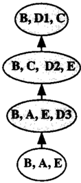
If the value sets are nested, that is, V1 2 . . . 2 Vm, then the rooted cluster tree shown in Figure lla is properly constructed. Otherwise, v;+1 � Vi+2 if and only if Vi+J n Vi + 2 = 0. Suppose that Vi+ I n v;+2 = 0 but v; 2 ( Vi + ! U Vi +2 ). In that case, then the partial tree shown in Figure llb is properly constructed. D

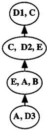
Of course, the purpose of this exercise is to generate more efficient rooted cluster trees. Examples of such for the influence diagrams from Section 2 are shown in Figure 12 and Figure 13. They are indeed more efficient than the rooted cluster trees in Figure 4 and Figure 5, respectively, reducing the size of the cluster state spaces.

The rest of this section contains the derivation of three simple but powerful results, based on the definition of properly constructed rooted cluster tree. First, the in­ wardmost cluster with a particular decision must con­ tain its requisite observations.

Lemma 1 (Current Requisite Observations) Given a rooted cluster tree properly constructed for

三

an influence diagram, all requisite observed variables for decision D are contained in the inwardmost clus­ ter containing D. Furthermore, any variables in both that cluster and the next inward cluster are observed when D is chosen.

Proof: By proper construction, any variable observed before D is chosen must be weakly inward of D and any requisite observation must be contained in a cluster with D. On the other hand, if A is not observed before D is chosen and strictly inward of D then it must not be contained in that cluster. 0

Next, when an uncertainty becomes observable before decision D is chosen, it will not become requisite unless it is weakly outward to D.

Theorem 2 (Newly Requisite Observations) Given a rooted cluster tree properly constructed for an influence diagram, if uncertainty A is not weakly out­ ward of decision D nor in any clusters with D then if A were to be observed before D were chosen it would not be requisite for D.

Proof: By proper construction and Lemma 1, the util­ ity from D is weakly outward from D and all variables in common between the inwardmost cluster containing D and the next inward cluster are observed when D is chosen. Therefore, the utility is separated in the clus­ ter tree from A by observations for D, and the utility from D is conditionally independent of A given the ob­ servations for D (Jensen and others 1990a; Lauritzen and others 1990). 0

Finally, when an uncertainty stops being observable before decision D is chosen, all of the observations now requisite for D are weakly inward.

Proposition 1 (Previously Requisite Observa­ tions) Given a rooted cluster tree properly constructed for an influence diagram where uncertainty A is ob­ served before decision D is chosen, then if A were not to be observed before D were chosen, all variables which would be requisite observations for D are weakly inward of D.

Proof: When properly constructed, all variables ob­ served before decision D is chosen (not just the requi­ site ones) are weakly inward of decision D. 0

5 Computing the Value of Information

The new results from Section 4 can now be applied to perform value of information calculations on the rooted cluster tree for the original influence diagram. First a method is presented for computing the value of a decision problem when an uncertainty is already observed. This is then generalized to computing the value when there is an earlier observation, and then when there is a later observation.

Suppose that an uncertainty has already been ob­ served, such as a in the influence diagram shown in Figure 3. By Theorem 2 it can be requisite only for decisions weakly inward in the tree shown in Figure 13. By exploiting the probabilistic heritage of the decision algorithm (Jensen and others 1990b; Lauritzen and Spiegelhalter 1988), the rooted cluster tree is ideally suited to solve this problem. First, the evidence is stored in the probability potential in a cluster contain­ ing a, say the inwardmost cluster containing a. Now Algorithm 1 could be run incorporating this evidence.

Suppose, however, that Algorithm 1 had already been run before a was observed. No problem-only the clus­ ters between the inwardmost cluster containing a and the root need to be visited. All of the other calcu­ lations are unchanged! We could perform this same operation even if a were not observed precisely, pro­ vided we had some imperfect observation about a rep­ resented by a likelihood function.

Now consider the case in which an uncertainty will be

observed earlier, but has not yet been observed, such as B in Figure 2. Again it is possible to exploit the well-known properties of cluster trees. To compute the value of the decision problem in which B will be ob­ served earlier, cycle through all of the possible values of B, performing the calculations each time as though B were observed. The potentials computed can then be summed, thereby incorporating the probability dis­ tribution over the different possible values of B. If this summing occurs immediately after the optimal policy for D; is computed, then this is the value of observing B before D; is chosen.

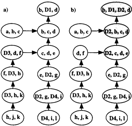
One can think of this as "effectively" adding B to the clusters inward to the inwardmost cluster containing D;, as shown in Figure 14. In Figure 14a, this is used to compute the value of observing B before D1, and in Figure 14b before D2. Figure 14c is not different from Figure 12 because B would not be requisite if it were observed before D3. This can be recognized immediately from the rooted cluster tree in Figure 12 in which B is inward of D3. Note that unlike Figure 4, in which the tree has been "expanded," this approach sums over cases, doing the same work, but there is no need to store the larger tables, and it uses the original rooted cluster tree!

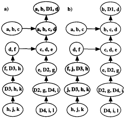
Now consider the influence diagram shown in Figure 3. Observing a earlier yields the effective rooted cluster tree shown in Figure 15a. Uncertainty a would be requisite for D1 but not for any of the later decisions. Suppose instead that j were observed earlier. It cannot be observed before D1 since it is a descendant of D1. It is not requisite for D2 or D4 since it is not inward of either, but it would be requisite for D3 as shown in Figure 15b.

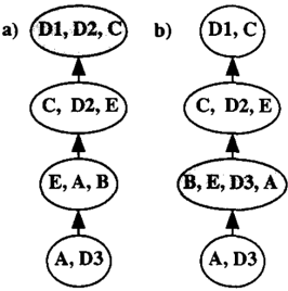
Now suppose that a variable is observed later rather than earlier. Consider C in Figure 1 and suppose that it is no longer observed before D2 is chosen. From Proposition 1, the observations now requisite for D2 are inward, so the solution is to run Algorithm 2 to

figure how inward D2 must effectively move up as in Figure 16a. Only now maximize over different cases for D2 instead of summing. Similarly, if A were not observed for D3, D3 can be effectively moved inward as in Figure 16b. Finally, if E were not observed for D3 there is no change, since E is not requisite for D3.

Finally, a similar process can be done for the diagram in Figure 3. Figure 17a shows the effective rooted clus­ ter tree when f is no longer observed before D3 and Figure 17b shows the effective tree when e is no longer observed before D2.

6 Conclusions and Future Research

This paper has developed improved value of informa­ tion calculations over previous work in two respects. First, it improves the rooted cluster trees used to solve

for the value of a decision problem. Second, it devel­ ops methods for reusing the original tree in order to perform multiple value of information calculations.

There are several opportunities for further research. When a particular variable is observed at multiple ear­ lier decisions it should be possible to reuse some of the calculations. Also, this approach exploits the special properties of changing the time when a single uncer­ tainty becomes observed. It would be useful if the method could be generalized to solve the decision prob­ lem with any set of informational assumptions from the original rooted cluster tree. If that could be done efficiently, then the original decision problem could be solved from the most convenient cluster tree.

Acknowledgments

This paper has benefited from the comments, sugges­ tions, and ideas of friends and students, most notably Mark Peot and Prakash Shenoy.

References

Dittmer, S. L. and F. Jensen. "Myopic Value of Infor­ mation in Influence Diagrams." In Uncertainty in Artificial Intelligence: Proceedings of the Thir­ teenth Conference, eds. D Geiger and P P Shenoy. 142-149. San Francisco, CA: Morgan Kaufmann, 1997.

Howard, R. A. and J. E. Matheson. "Influence Dia­ grams." In The Principles and Applications of Decision Analysis, eds. R. A. Howard and J. E. Matheson. II. Menlo Park, CA: Strategic Decisions Group, 1984.

Jensen, F., F. V. Jensen, and S. L. Dittmer. "From

Influence Diagrams to Junction Trees." In Uncer­ tainty in Artificial Intelligence: Proceedings of the Tenth Conference, eds. R Lopez de Mantaras and D Poole. 367-373. San Mateo, CA: Morgan Kauf­ mann, 1994.

Jensen, F. V., S. L. Lauritzen, and K. G. Olesen. "Bayesian Updating in Causal Probabilistic Networks by Local Computations." Comp. Stats. Q. 4 ( 1990a ) : 269-282.

Jensen, F. V., K. G. Olesen, and S. K. Andersen. "An algebra of Bayesian belief universes for knowledge based systems." Networks 20 ( 1990b ) : 637-659.

Lauritzen, S. L., A. P. Dawid, B. N. Larsen, and H.-G. Leimer. "Independence properties of directed Markov fields." Networks 20 ( 1990 ) : 491-505.

Lauritzen, S. L. and D. J. Spiegelhalter. "Local com­ putations with probabilities on graphical structures and their application to expert systems." JRSS B 50 ( 2 1988 ) : 157-224.

Ndilikilikesha, P. Potential Influence Diagrams. University of Kansas, School of Business, 1991. Work­ ing Paper 235.

Raiffa, H. Decision Analysis. Addison-Wesley, 1968. Reading, MA:

Shachter, R. D. "Evaluating Influence Diagrams." Ops. Rsrch. 34 ( November-December 1986 ) : 871882.

Shachter, R. D. "Bayes-Ball: The Rational Pastime ( for Determining Irrelevance and Requisite Informa­ tion in Belief Networks and Influence Diagrams ) ." In Uncertainty in Artificial Intelligence: Proceed­ ings of the Fourteenth Conference, 480-487. San Francisco, CA: Morgan Kaufmann, 1998.

Shachter, R. D. and P. M. Ndilikilikesha. "Using Po­ tential Influence Diagrams for Probabilistic Inference and Decision Making." In Uncertainty in Artificial Intelligence: Proceedings of the Ninth Confer­ ence, 383-390. San Mateo, CA: Morgan Kaufmann, 1993.

Shachter, R. D. and M. A. Peot. "Decision Making Using Probabilistic Inference Methods." In Uncer­ tainty in Artificial Intelligence: Proceedings of the Eighth Conference, 276-283. San Mateo, CA: Morgan Kaufmann, 1992.

Shenoy, P. P. "Valuation-Based Systems for Bayesian Decision Analysis." Ops. Rsrch. 40 ( 3 1992 ) : 463484.

Tatman, J. A. and R. D. Shachter. "Dynamic Pro­ gramming and Influence Diagrams." IEEE SMC 20 ( 2 1990 ) : 365-379.