End-User Construction of Influence Diagrams for Bayesian Statistics

Harold P. Lehmann, MD PhD

Johns Hopkins University Baltimore, MD 21205

Iehmann @welchgate.welch.jhu.edu

Abstract

Influence diagrams are ideal knowledge representations for Bayesian statistical models. However, these diagrams are difficult for end users to interpret and to manipulate. We present a user-based architecture that enables end users to create and to manipulate the knowledge representation. We use the problem of physicians' interpretation of two-arm parallel randomized clinical trials (T APRCT) to illustrate the architecture and its use. There are three primary data structures. Elements of statistical models are encoded as subgraphs of a restricted class of influence diagram. The interpretations of those elements are mapped into users' language in a domain-specific, user-based semantic interface, called a patient-flow diagram, in the T APRCT problem. Pennitted transformations of the statistical model that maintain the semantic relationships of the model are encoded in a metadata-state diagram, called the cohort-state diagram, in the T APRCT problem. The algorithm that runs the system uses modular actions called construction steps. This framework has been implemented in a system called THOMAS, that allows physicians to interpret the data reported from a T APR CT. Keywords: statistics, Bayesian, expert systems, artificial intelligence, influence diagrams, probabilistic reasoning, knowledge acquisition, clinical trials.

1 INTRODUCTION

Dynamic construction of influence diagrams is a powerful strategy for enabling a computer-based system to match a human's knowledge. During statistical analysis, the analyst creates a model of the domain and of the data, so such dynamic construction is crucial when creating intelligent systems for statistical analysis. Influence diagrams are ideal knowledge representations for statistical models, especially for Bayesian statistical models (Smith 1989). However, the use of Bayesian statistics needs the end user to direct much of the analysis, because of the

Ross D. Shachter, PhD Stanford University Stanford, CA 94305 [email protected] importance of the user's prior knowledge of the domain. Unfortunately, by the very nature of the complexity and technicality of Bayesian statistical models, the typical end

structures of these models or the implications of any choices for important issues like methodological concerns or prior knowledge.

Our thesis is that a user-based semantic interface to influence-diagram construction will allow such users to perform a meaningful Bayesian-statistical analysis. We shall demonstrate a program architecture we call user based (UB) that can serve as the basis for building a wide variety of such systems. We shall target a particular user community throughout this paper: physician readers of reports of clinical trials, specifically, two-arm parallel ran-

Table 1: Elements of the influence-diagram representation of statistical models.

Object	Class	Influence-Diagram Element	Statistical-Model Interpretation
Level		Population	Generalknowledge
		Sample	Study-specific knowledge
		Effective	Measuredknowledge
		Patient	Patient-specific knowledge
N<XIe		Outcome	e.g., Lifespan
		Parameter
		Outcome	e.g., Mortality rate
		Methodological	e. g., Withdrawal rate
Arc		Interlevel
		Population---7 Study	External validity e.g., Selection bias
		Study ---7 Effective	Measurement reliability e.g., Specificity
		Isotypal
		Population ---7 population	Domainknowledge e.g., Placebo population mortality rate = baseline population mortality rate
		Sample ---7 sample	Internal validity e.g., Withdrawal model
		Methodological ---7 outcome	Specific relationships e. g., Mixture models

domized clinical trials (T APRCT). These are studies where patients are randomly assigned to one of two therapies; often, one of them is a placebo control treatment. The principles of using the architecture, however, are genetic.

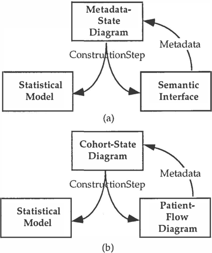
Fig. 1 depicts the architecture. In Section 2, we shall discuss statistical models, in Section 3, the semantic interface, in Section 4, metadata and the metadata-SL:'lte diagram, and in Section 5, the construction steps. � n Section 6, we shall discuss an implementation of tl11s architecture, in Section , ? we discuss previous work, and conclude in Section 8.

2 STATISTICAL MODEL

A statistical model comprises elements, interpretations, and transformations. Elements of a statistical model include: probability models, parameters, observations, and assumptions that allow the analyst to relate tl1e observations to the parameters. Interpretations map elements of the statistical model into inferential concems in the world. Transformations are the permitted operations that change the statistical model, while maintaining tl1e interpretations of the model.

In the UB m·chitecture, we use influence diagrams (Howard and Matheson 1981; Oliver and Smith 1990) to represent the elements of statistical models (Smith 1989). As generally described, there m-e two classes of o�jects in these acyclic, directed graphs. Nodes are the objects of interest: pm-ameters, observations, decision options and decision objectives. Note that parameters and observations m-e continuous quantities, unlike the discrete variables for which influence diagrams have been traditionally used in AI systems. Arcs are objects representing dependencies; tl1e absence of an m-c between two nodes denotes the independence of tl1e vatiables those nodes represent.

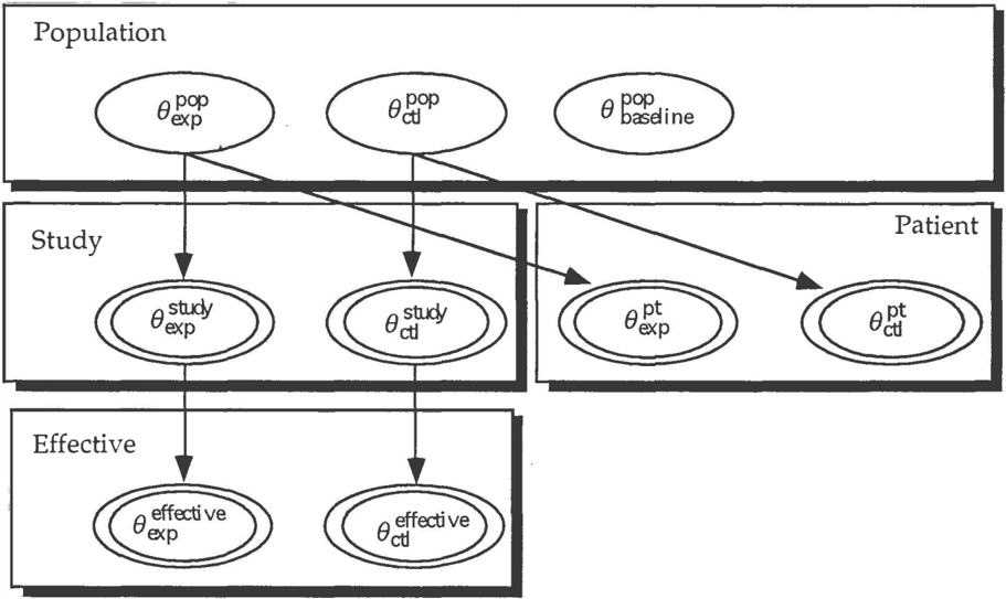
To aid t11e communication with users, we add level as a third object. Levels m-e elements that contain nodes and give tl10se nodes interpretive semantics (e.g., population mortality rate as opposed to sample mortality rate). Levels limit the transformative interactions among pm·mneters. The specific levels we use for the T APRCT problem m·e as follows (see Table 1): effective level allows for modeling concerns regm-ding measurement reliability; t11e sample level allows for modeling concems regm·ding intemal validity; the population level allows for modeling concerns regarding extemal validity; and the patient level allows us to represent differences between the patient and the population. Fig. 2 depicts the initial influence-diagram of the statistical model for the T APRCT problem.

In the UB m-chitecture, we m-e concerned primru-ily with transformations tlwt signify methodological concems noted by the reader of t11e study report. We use construction steps tlmt transform tl1e statistical model to comply with the interpretative meaning of the methodological concern (see Section 5). The steps m-e moduhu· statements of permitted transformations. This modulm·ity will allow tl1e user to take as much charge of the interaction with the machine as possible. Note that modification of a statistical model is, by definition, model dliven; t11e nature of the model permits or forbids different types of modification.

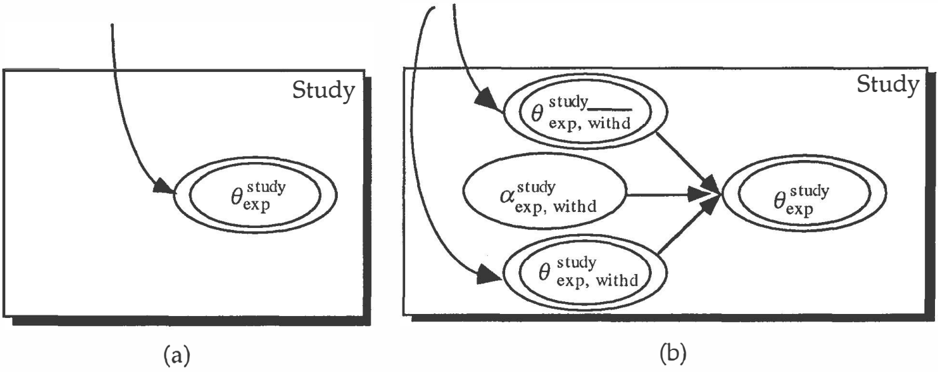
Fig. 3 exhibits the representation of a particular bias in an T APRCT, showing a part of t11e influence-diagram representation of a trial before and after the construction step of including the methodological concern of withdrawall (for simplicity, only the study level is shown). The construction has remodeled the dependence of the study parameter: no longer identical to a population parameter (t11e initial, default relationship), it is now a function of a mixture of other parameters.2 The mixture parameter represents t11e witl1drawal rate. In a classical-statistical system, its value would be estimated from tlle data in tlle study. In a B ayesian system, its value would depend on the prior belief of the analyst­ what witlldrawal rate she would expect in t11is type of study-as well as on the data observed. The modular concept for tllis bias is tlle recognition tlmt withdrawals affects tlle study parameter only, and in a particular way.

1 Withdrawal refers to patients who no longer follow the study protocol, but about whom outcome data are known.

2Left out of Fig. 2 are the dependencies of the other study parameters on particular population parameters. For instance, the outcome study parameter in patients assigned to experimental treatment but who withdrew from therapy is made functionally identical on the standard­ care population parameter.

3 SEMANTIC INTERFACE: THE PATIENT-FLOW DIAGRAM

Most statistical clients require an interface tllat translates elements of a statistical model into a language whose semantics tlley understand. For tlle UB architecture, we chose as t11e metaphor for tlle semantic interface tlle patient-flow diagram. In such a diagram, children nodes represent cohort at a particular point in time. Modification of a cohort is akin to a traversal from one state of knowledge to cohorts of patien� whose numbers sum to that of the parent node, but each of whom experienced an important different event in tlle study. A patient-flow diagram depicts the history of patients in tlle course of a study and is often published in a report of a clinical trial. Users manipulate t11e statistical model by m�mipulating the patient-flow diagram-tlle domain-based metaphor. For instance, t11ey might select a cohort and communicate (e.g., via a pop-up menu) that some patients in tlle cohort witlldrew from tlle assigned tllerapy. Note t11at, in contrast to the statistical model, modification of the patient-flow diagram is data driven.

4 METADATA-STATE DIAGRAM: THE COHORT-STATE DIAGRAM

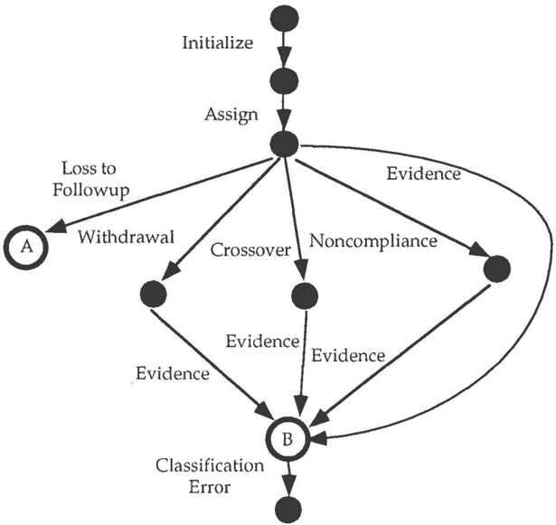
The metadata-state diagram (MDSD) mediates between the user's data-driven manipulation of the patient-flow term refers to knowledge about what sorts of information are contained in cohorts and in nodes, and what modifications are permitted. The MDSD for the T APRCT problem is called the cohort-state diagram. (see Fig. 4). The state in this diagram refers to the state of knowledge regarding a another; implementing that change of state results in changing the statistical model, as well as the patient-flow diagram. The diagram aspect of the MDSD is the set of path traversals permitted. For the T APRCT problem, it represents, fm' instance, the methodological knowledge (based on the definition of loss to followup) that if a statistical model currently reflects the fact that a cohort of patients has been lost to followup, then the user's .attempt to provide evidence about that cohort should be denied; tile traversal fmm state A to B in Fig. 4 is forbidden.

In summary, a cohort in the patient-flow diagnun points to a state in the metadata-state diagram. The cohort also points to study and effective outcome parameters (such as mortality rates) in the influence diagram (statistical model). Evidence within a cohort becomes a node in the influence diagram, dependent on the effective outcome parameter associated with tile cohort. The relationship between population outcome parameter and study outcome parameter reflects domain knowledge.

diagram and the program model-driven modification of the statistical model. Metadata refers to information about data (Chytil 1986). In the UB architecture, this

5 CONSTRUCTION STEPS

The top-level controlling algorithm works as follows: The user completes an interaction with the patient-flow diagram. The patient-flow diagram then translates the user's metadata directive into a machine-usable format that includes the metadatum and the target cohort. Unless the directive signals tetmination of the modeling process, the system examines the cohort-state diagram to determine whether tile directive is pennitted, by inspecting the arcs emanating from the target cohort's state in the diagram. If the directive is permitted, the system then executes the corresponding construction step, modifying the patient­ flow diagram and the statistical model in the process. If new statistical parentless parameters are created by the construction step, the user is asked to assess prior beliefs about those parameters; the constructed names of the parameters are meaningful to the physician user.

Names for new parameters are created by concatenating phrases associated with transitions in the metadata-state diagram, modified by knowledge available to the system regarding the target cohort. For instance, a new withdrawal-cohort study outcome parameter will be called study <outcome> <parameter type> for patients who withdrew from therapy in <name of parental cohort>, where <outcome> might be mortality, <parameter type>

might be rate, and <name of parental cohort> is available from the patient-flow diagram.

As an example, consider the pseudocode for the withdraw-transition. There are two major methods for this object: pfd-action and sm-action, corresponding to the construction steps performed on the patient-flow diagram and on the statistical model, respectively.

(method pfd-action (withdraw-transition, source-cohort) withdraw-cohort (create-cohort(yes) no-withdraw-cohort (create-cohort(no) connect (source-cohort, withdraw-cohort) connect (source-cohort, no-withdrawcohort) treatment (withdraw-cohort (source-cohort)) (-baseline-treatment )

Two new cohorts ru·e created, with differing semantics as regards the withdrawal status of patients in those cohorts. The cohorts are then incorporated into the patient-now diagram. Finally, an element of domain knowledge is included, that withdrawn patients effectively receive baseline care.

(method sm-action(withdraw-transition, source­ cohort) alpha (create-mixing-parameter(sout·ce­ cohort) withdraw-outcome-parameter (outcome­ parameter(withdraw-cohort(source­ cohort)) no-withdraw-outcome-pat·ameter (­ outcome-parameter(no-withdraw-cohort (source-cohort)) make-mixture(source-cohort-outcome­ parameter, alpha, withdraw-outcome-parameter, no-withdraw-outcome-parameter) make-identical( withdraw-outcome-parameter, population-baseline-outcome-parameter) make-identical(no-withdraw-outcome parameter ,population-outcome­ parameter(treatment(source-cohort))))

Here, the mtxmg model of Fig. 3 is created. The parameters here are all at the srunple level; the functions that find the study-level parameters have been eliminated for the sake of simplicity. The action, make-mixture, is here performing the main work, converting a parameter (source-cohort-outcome-parameter) formerly identical to a population-level parameter into one that is a deterministic function of other parameters. Domain knowledge in encoded in the instruction to make, the newly created study-level outcome parameters identically deterministic on outcome parameters in the population level,.

6 IMPLEMENTATION

The architecture presented here has been implemented in a system called THOMAS (Lehmann 1991), that focuses on problems of intemal validity in T APRCT studies. The int1uence diagrams are restricted to having one layer of marginally independent chance nodes whose pdfs are beta distributions. All other nodes are deterministic or evidential. Evidence nodes have only one parent. The construction steps are modules whose statistical components are based on the methodological models of Eddy, et al. (Eddy, Hasselblad et al. 1991).

The primary outputs are posterior distributions for the parameters of the model, and expected utility (life expectancy). The algorithm for calculating posterior probabilities uses posterior-mode detetmination, based on modified Newton-Raphson steepest descent (Shachter 1990), using the approach of Berndt and colleagues (Berndt, Hall et al. 1974). This algorithm requires matrix inversion, an 0(m3) process, where m is the number of parameters with no parents. In our use of this algorithm, parameters that are functionally identical to other parameters are eliminated from the model in O(n) time prior to the posterior-mode determination, where n is the number of statistical parameters. Thus, the overhead of maintaining the influence-diagrrun levels takes little away from the performance of the algoritlun.

Calculation of expected utility is through unidimensional integration.

THOMAS is implemented on a Macintosh II computer. The patient-flow diagram was written in HyperTalk and the remainder of the system was written in Macintosh Common Lisp, using the Cmnmon Lisp Object System to house the various objects in the UB architecture. Communication between the t wo systems used TalkToMe, a precursor to AppleEvents.

A number of different MDSDs and different patient-flow diagrams were tested in this architecture. In each experiment, and as desired, modifications of a major structure did not require changes in the other structure.

A small number of clinicians used THOMAS as intended. The needed tasks were conceptually familiar. Some users disliked the navigational interface, but found the patient­ flow diagram to be self-evident (as we expected).

7 OTHER WORK

This work reflects on research in the AI-and-stati�tics community, in the biostatistical community, and in the AI-and-uncertainty community. Statisticians applying AI In the biostatistical community, Hasselblad and Eddy have developed the F AST*PRO program (associated wit11 (Eddy, Hasselblad et al. 1991)) to allow medical researchers construct influence diagrams that represent statistical models. Differences with our work include their focus on the data-driven direction of influence-diagram construction and their lack of a semantic inte1face.

Finally, various researchers of AI and uncertainty have built systems that automatically build influence diagrams. Goldman and Chamiak (Goldman and Chamiak 1990) have developed a language for constructing influence diagrams, specifically for the domain of natural-language processing. Their system uses a hienu·chical and typed influence diagram, as we do; their construction algorithm is more model-driven than is ours. Similarly, Breese (Breese 1987) has built a system that constructs influence diagrams out of modular components. However, he techniques to statistical problems have, by and large, focused on helping the statistical analyst, rather than the end user (Nelde and Wolstenhome 1986; Lubinsky 1987; Oldford and Peters 1988).

requires the user to have a greater knowledge of influence diagrmns t11m1 we do.

8 CONCLUSION

We have presented an architecture for creating tools that allow end users to interpret t11e results of scientific studies whose data requires statistical analysis for interpretation. This architecture implements the general decision-analytic approach to scientific inference presented by Lehmann (Lehmann 1990). We believe that this architecture could be extended for other data-analysis problems. For instance, for crossover studies, where patients are first given one, then anot11er treatment, the MDSD and the patient-flow diagram would both have to be modified. Furthermore, t11e m·chitecture could be extended to account for other methodological concerns. For instance, randomization is a key consideration whose goal is to

assure similarity of treatment groups. This concern can be represented at the sample level in tenus of relative occurrences of covariate states for study subjects in every treatment ann, and in tenns of their relative contributions.

Even more generally, we might imagine that this architecture would be suitable for other AI domains where the primary user (or even knowledge engineer) may wish to be protected from details of Bayesian modeling. Thus, in a vision system, the cognate of the patient-flow diagram might be the hierarchy of visual perception that Levitt and colleagues (Binford, Levitt et al. 1987) have put to such good use, while the MDSD might represent pennitted, meaningful sequences of visual processing. Each limb of transition in that process would have implications for the underlying influence diagram as well as for an interface that a user would face.

In each case, there are several tasks for the knowledge engineer. First, he must decide the propriety of the architecture. Second, from observation of users, he must decide on the appropriate semantic metaphor and on tl1e central object of manipulation. Third, from discussions with domain experts, he must encode the rules for transitions. Finally, he must figure out what influence diagram structures and transformations embody the experts' intentions. This overall construction task is far from being automated.

In summary, statisticians confront the same problem that Al-system designers do: How should valid inferences be made from real-world data? The user-bao;;ed architecture can be of service to both these communities.

Acknowledgments

We thank Bill Brown for his statistical expertise and criticism in our constructing THOMAS, Bill Poland for his help in programming THOMAS, Ruben Kleiman, of Apple Computers for supplying TalkToMe, and Ted Shortliffe, Brad Farr, Holly Jimison, and Eddie Herskovits for constructive discussions in the course of this work. This work was funded by NLM grant LM07033.

References

• Berndt, E. K., B. H. Hall, et al. (1974). "Estimation and inference in nonlinear structural models." Annals of Economic and Social Measurement 3/4: 653-665.
• Binford, T. 0., T. S. Levitt, et al. (1987). Bayesian inference in model-based machine vision. Proceedings of the Third Annual Workshop on Uncertainty in Artiticial Intelligence, University of Washington, July 10-12,
• Breese, J. (1987). Knowledge representation and inference in intelligent decision systems. Department of Engineering-Economic Systems, Stanford University.
• Chytil, M. K. (1986). Metadata and its role in medical informatics. MEDINFO 86, North-Holland.
• Eddy, D. M., V. Hasselblad, et al. (1991). The statistical synthesis of evidence: Meta-analysis by the Confidence Profile Method. Boston, Academic Press.
• Goldman, R. P. and E. Charniak (1990). Dynamic construction of belief networks. Proceedings of the Sixth Annual Workshop on Uncertainty in Artificial Intelligence, Cambridge, MA, July 27-29,
• Howard, R. A. and J. E. Matheson (1981). Readings on the Principles and Applications of Decision Analysis. Menlo Park, CA, Strategic Decision Group.
• Lehmann, H. P. (1990). A decision-theoretic model for using scientific data. Uncertainty in artificial intelligence 5, Amsterdam, Nmth-Holland.
• Lehmann, H. P. (1991). A Bayesian Computer-Based Approach to the Physician's Use of the Clinical Research Literature. Stanford University.
• Lubinsky, D. J. (1987). TESS: A tree-based environment for statistical strategies. COMPSTAT-87,
• Nelde, J. A. and D. Wolstenhome (1986). A front-end for GLIM. COMPST AT -86, Fort Collins, CO,
• Oldford, R. W. and S. C. Peters (1988). "DINDE: Towards more sophisticated software environments for statistics." SIAM Journal of Scientific and Statistical Computing 9: 191-211.
• Oliver, R. M. and J. Q. Smith (1990). Influence diagrams, belief nets, and decision analysis. Chichester, Wiley.
• Shachter, R. D. (1990). Posterior mode analysis. Influence diagrams, belief nets, and decision analysis. R. M. 0. a. J. Q. Smitl1. London, Wiley & Sons.
• Smith, J. Q. (1989). "Influence Diagrams for Statistical Modeling." The Annals of Statistics 17(2): 654-672.