Error Estimation in Approximate Bayesian Belief Network Inference

Enrique F. Castillo Applied Mathematics Dept University of Cantabria 39005 Santander, Spain castie@ccaix3. unican.es

Remco R. Bouckaert Computer Science Dept. Utrecht University The Netherlands [email protected]

Abstract

We can perform inference in Bayesian be­ lief networks by enumerating instantiations with high probability thus approximating the marginals. In this paper, we present a method for determining the fraction of in­ stantiations that has to be considered such that the absolute error in the marginals does not exceed a predefined value. The method is based on extreme value theory. Essentially, the proposed method uses the reversed gener­ alized Pareto distribution to model probabili­ ties of instantiations below a given threshold. Based on this distribution, an estimate of the maximal absolute error if instantiations with probability smaller than u are disregarded can be made.

1 INTRODUCTION

When propagating uncertainty in Bayesian networks, one has to account for the probabilities of certain events. In general, most events have a very small prob­ ability of occurrence and the sum of the probabilities of rare events is negligible. Many techniques applied to Bayesian belief networks rely on this assumption. For example, various approximation algorithms for in­ ference [5, 13, 16, 15] and caching of probabilities of likely events [14] are founded on this assumption. In this paper we concentrate on the error obtained in ap­ proximating marginal probabilities.

However, on fore-hand it is not known what the to­ tal contribution of the events with low probability to the marginals is. As a result, it is difficult to speak in terms of absolute error-bounds. On the other hand, if we know on fore-hand what the total contribution of the events with probability smaller than q is to the marginals, we can calculate, for example, the number of iterations of simulation algorithms when a certain error-bound is demanded. A variant of stratified simu­ lation [3, 4] is guaranteed to visit all events with prob­ ability larger than 1/m where m is the number of it-

Jose M. Sarabia University of Cantabria

Economics Dept. 39005 Santander, Spain

Cristina Solares Applied Mathematics Dept. University of Cantabria

39005 Santander, Spain erations. Furthermore, we can determine a reasonable size of a cache as proposed in [14].

Druzdzel [12] gave a solution for the problem by defin­ ing a random variable X as the logarithm of the proba­ bilities of an event and selecting events with a uniform distribution. He showed that under some general con­ ditions the distribution over X can be approximated by a log-normal distribution. From this distribution, an estimate can be made of the total contribution of the events with probability smaller than q to the marginals.

However, the log-normal approximation is based on the central limit theorem. As a result, the approxima­ tion is good in the neighborhood of the mean of X. But we are interested in the tails of the distribution over X, where the log-normal approximation can dif­ ferentiate considerably from the real distribution. In fact, estimates based on the log-normal approximation differ so much that reliable estimates are not possible for the tails.

An alternative for the log-normal approximation is ex­ treme value theory [6]. This theory is engaged with the tails (right or left) of distributions. In this paper, we define a random variable X as the probabilities of events and select events with a distribution propor­ tional to the probability of their occurrence. Note that we do not take the logarithm as [12] does, though we can work with logarithms as well with a small change in the interpretation of our model. We show how to approximate the left tail of the distribution over X, which gives us the total contribution of the events with probability smaller than q to the marginals. Our the­ ory applies to distributions involving continuous vari­ ables and gives a very good approximation for discrete variables.

In Section 2 we give a formal statement of the prob­ lem and some definitions. In Section 3 we present our model for solving the problem and in Section 4 we show how to estimate the various parameters of the model. We performed some experiments to get insight in the usability of our method. The results are presented in Section 5. Finally, in Section 6 we make some conclud­ ing remarks.

2 STATEMENT OF THE PROBLEM

A Bayesian belief network B over a set of variables V {x11 ... , Xn } is a pair (Bs, Bp ) , where Bs is a directed acyclic graph over V and B p is the set of conditional probabilities of Xi given its parents 1ri· A Bayesian belief network defines a probability distribution [17] over V PB(V) = TI� 1 P(x;!1ri)·

Inference in such knowledge based systems over V consists of the calculations for each xi E V of the marginals P(xiiE) Z:::x1EV\Exi PB(VIE) where val­ ues of certain variables E c V are known to have values ei for Xi E E. For ease of exposition, we as­ sume that E = 0, that is, that there is no evidence. Since the above summation is computational infeasi­ ble when n is large, the marginal can be approximated by summing over a subset of instantiations of V with high probability. We are interested in calculating the error that occurs in such an approximation. More spe­ cific, we are interested in determining the contribution of all instantiations with probability smaller than q to the total probability mass,

For continuous variables, consider the function P I v --+ JR+, defined as

where Iv is the set of all possible instantiations of the set V, and JR+ is the set of all non-negative real numbers, that is, we associate with each instantiation its probability density function ( pdf) value. Assum­ ing some regularity conditions, P is a unidimensional random variable.

Let f ( p ) be the probability density function of P. The elemental contribution of all instantiations with prob­ ability p :::; P :::; p + d p to the total probability mass is p f (p ) d p . Further, the fraction of the contribution of all instantiations with probability smaller than q to the total probability mass becomes

where the denominator is the expected value of P and we have made the change of variable u = F (p ) , where F ( p ) is the cumulative density function ( cdf) of P, to get the right-hand side expression. Note that G(q) is the Lorenz curve of P ([1, 2, 11, 10], which is a cdf that can be associated with a new random variable Q with the same domain as P.

Alternatively, we can write the Lorenz curve in terms of the proportion r of instantiations contributing a given fraction of the total probability mass, by making the extra change of variable r F(q) to get

where L(r) is a cdf with associated domain [0, 1J. How­ ever, in this paper we shall use the Lorenz curve (2).

Assume that we consider the subset Vp0 of all instan­ tiations with associated p values such that p ?:: P o and we calculate marginal probabilities based on this sub­ set Vvo· instead of the set V. Then, G(Po) is an up­ per bound for the error of the marginal probabilities. Thus, we can take G as the basis for error estimation.

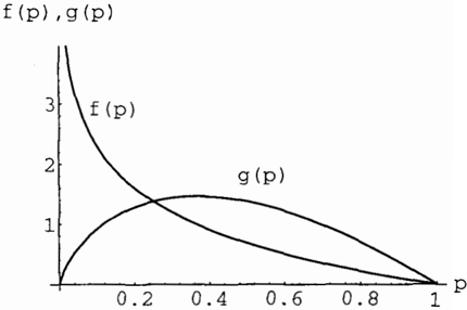
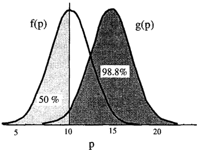
For example, Figure 1 shows both densities f (p ) and g(p), where f (p) is the density of P and g(p) the den­ sity of the contribution to the total probability mass of instantiations with associated probability p. Now 50 %of the instantiations, i.e., instantiations with as­ sociated probability P > 10, contribute 98.8 % to the total probability mass (the area below the g function in the region P > 10). Consequently, consideration of only these instantiations leads to a maximum error of 0.012 in any probability evaluation.

p

Figure 1: illustration of how 50 % of the instantiations can contribute 98.8 % to the total probability mass.

The problem that we consider in this paper is the ap­ proximation of G. More precisely, we try to estimate the left tail of G.

3 PROPOSED MODEL

Thus, we are not interested in estimating f (p) but the curve G(q) of P, or to be more precise its left tail. Due to the fact that we want small errors in the evalu­ ation of marginal probabilities, we consider neglecting a small fraction of the probability mass, that is, we re­ ally want to estimate lower percentiles of G(q). Thus, we must deal with the left tail of the associated dis­ tribution G(q). This could be achieved by randomly

generating a sample for G and straightforward estima­ tion. It is well known that in order to get an estimate of a small proportion p with a given relative error, the required sample size is proportional to 1 / p. Since p is very small in our case, a very large sample would be necessary. An alternative is to use extreme value theory.

To apply extreme value theory, we consider the ran­ dom variable Q with associated cdf G(q). We trans­ form Q by truncating it at a threshold value u and then translating the origin to u, thus getting a new random variable S, which is defined as Q -u given Q :::; u. The random variable S has the cdf H(s; u) which is

for q0 -u :::; s:::; 0, where G(q) is the cdf of Q and Qo is the lower endpoint of G or F.

It follows from ( 4) that G(q) for small values of p can be written as

Thus, estimating G(q) is equivalent to estimating: (a) G(u) and (b) H(q-u;u). We discuss these two points in the following paragraphs.

To choose H(q-u; u), we use the Reversed Generalized Pareto Distribution (RGPD), which will be justified by Theorem 1. The RGPD U(z; b, a) is a distribution defined by

where b and a are the scale and shape parameters, respectively.

Theorem 1 The RGPD U(q; b, a) is a good a p proxi­ mation of H ( q; u), in the sense that

for some fixed a and functions b ( u), if and only if H is in the minimal domain of attraction of one extreme value distribution.

Note that practically all cdfs used in textbooks satisfy this condition. See Pickands [18] for a proof of the equivalent result for the maximal domain of attrac­ tion. Using Theorem 1, from (5) and (6), the proposed model for the left tail of Q is

which depends on G(u) and two parameters b and a for each threshold value u.

4 ESTIMATION OF THE MODEL

The main problem for estimating b and a is that the associated random variables S and Q are not directly observable. However, we can observe P and obtain an ordered sample ( p1, . . . , pn)· A natural estimator for G(q) based on this sample is

for the discrete case and

for the continuous case. To estimate G(q) for q < u, one needs both G ( u) and H ( q -u; u). In practice, dif­ ferent values of u should be tried out and G(u) can be estimated by (9) and (10) for the discrete and contin­ uous case, respectively.

For estimating b and a we use the method proposed by Castillo et al. [7, 8, 9].

Let I = { i, j}, i < j E { 1, . . . , n}, then we have for the discrete case

and for the continuous case

Substituting (6) in both (11) and (12) and taking the logarithm1, we obtain

for the discrete and continuous case, respectively. It can be seen that (13) is a system of two equations in two unknowns, band a. Eliminating a, we obtain

We now show that the above estimators are well de­ fined, that is, (14) has one more solution in addition to the trivial solutions b = ±oo, a = 0.

1 We use the natural logarithm throughout this article.

Theorem 2 Equation {14} has a finite solution, in the interval (8o,O) if Ci(u-pj) -Cj(u- pi) > 0, or in the interval ( u - pi, 8o) if Ci(u- Pj)- Cj(u-Pi) <= 0, where

A proof of Theorem 2, which is given in the Appendix, is constructive for it gives rise to the following algo­ rithm for solving (14) for 8. Equation (14) is a func­ tion of only one variable, hence it can be solved easily using the bisection method as outlined in Theorem 1 and Algorithms I and II below. Thus, using Algorithm I, one can solve (14), for 8 and obtain an estimate of 8, 6 ( i, j), say. This estimate is then substituted in one of the two equations in (13) to obtain a corresponding estimate of o:, a(i ,j ) , which is given by

Algorithm I( p, i, j) {p is an array with ordered sam­ ples and i and j two indices}

1. Compute Ci and Cj and let d = Ci(u- pj)­ Cj(u-Pi)

2. case

• d = 0: b(i ,j ) = ±oo. This means a(i ,j ) = 0.
• d < 0: Use the bisection method on the in­ terval [u- Pi,8o], where 8o = (Ci-Cj)(uPi)(u-Pj)/d, to obtain a solution b(i ,j ) of (14)
• d > 0: Use the bisection method on the in­ terval [8o, 0] , where 8o = ( Ci -Cj )(u- pi)(uPj)/d, to obtain a solution b(i ,j ) of (14).

end case

1. Use b(i,j) to compute a(i,j) using (16).

4.1 FINAL ESTIMATES

The estimates found by Algorithm I are based on only two order statistics {Pi:n,Pj:n}, thus they do not uti­ lize the information contained in other order statistics. Statistically more efficient estimates are obtained us­ ing the following algorithm.

Algorithm II

1. Use Algorithm I to compute b(i ,j ) and &(i , j ) , where i = m/10; j = i + 1, . . . , m -1 and m is the number of data points below the threshold u.
2. Apply a robust function R(. ) to each of the above sets of estimates and obtain a corresponding over­ all estimates of 8 and o:.

Examples of the robust function, R(. ) in Step 2, in­ clude the median and the least median of squares

(LMS), Rousseeuw [19]. Thus, overall estimates of 8 and o: can be defined as or

where median(yi, Y2, . . . , Yn) is the median of {yl , Y2, . . . , Yn}, and LMS(yi, Y2, . . . , Yn) is the esti­ mate obtained using the LMS methods, which in this case is equal to the midpoint of the shortest inter­ val containing half of the numbers y1, y2, . . . , Yn (see Rousseeuw and Leroy [20], pp. 169).

5 EXPERIMENTS

We performed some experiments to get an impression of the applicability of our model. Further we compared the quality of our estimates with those based on the log-normal approximation [12].

First, we generated randomly a Bayesian belief net­ work over 15 binary variables as in [3]. We did not use larger networks in order to be able to determine exact values of G. The probability table are selected once using a uniform distribution over the unit interval and once using a uniform distribution over the inter­ val [0, 0.1] U [0.9, 1]. With this network, we generated a sample of 1000 cases using logic sampling [13]. This sample was used to estimate 8 and o: using algorithm II with the median as robust function. An exact calcu­ lation of G was performed by enumerating all instanti­ ations of the 15 variables and counting corresponding probabilities. For comparison the accumulated prob­ ability estimated based on the log-normal approximation J�o!q N(JL, a)/ f�ao N(JL, a) was calculated. The mean JL and variance a of the log-normal approxima­ tion were calculated exactly.

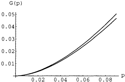
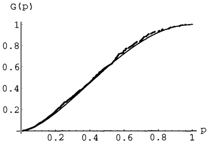
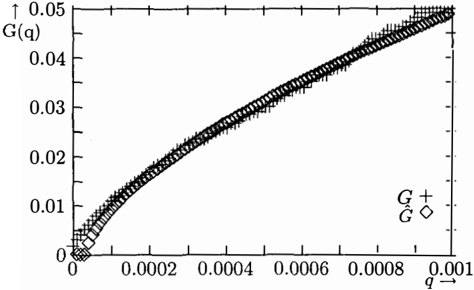
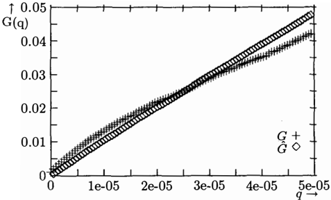
Figure 2 and 3 show the exact values of G together with its approximations based on Formula 8 for net­ work with probability tables selected from [0 .. 1] with u = 0.00005 and from [0, 0.1] U [0.9, 1] with u = 0.001, respectively. The value of u was obtained by starting with u = 0.005 and consecutively lowering u until the estimates of o: and 8 were based on about 50 cases. The y-axis shows the accumulated probability and the x-axis the values of q .

From the figure is clear that the approximation G dif­ fers only slightly from the exact values of G. So, the presented theory seems to give a good approximation. On the other hand, the approximation based on the log-normal distribution has a very large error; when applying this approximation we found that already at q = 5.10 - 6 the error is larger than 0.9 for both cases rendering it inapplicable for estimating G.

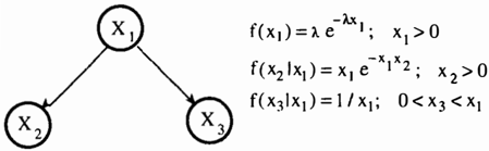
We also performed experiments with a belief network with continuous variables. Let V = {X1,X2,X3} and

consider the Bayesian belief network (Bs,Bp) in Fig­ ure 4. Then, we have P = f(xl)f(x2lxl)f(x31xl), so P = Aexp(-Axl)exp(-xlx2); x1,x2 > 0, 0 < X3 <

The exact distribution of the random variable P can be calculated as follows:

• First we consider the change of variable:

• Next we obtain the joint density of (P, U):

• Finally, we obtain the P-marginal:

with cdf

Then and

Figure 5 shows f( p) and the normalized g( p), which is the pdf associated with G(p), for A = 1 . From this we can find that 32% of the instantiations contribute 0.05% of the total probability.

p

We can simulate (X1, X2, X3) using the conditional probabilities in Figure 4. We have simulated a sample of size 1000, which is shown in Figure 6.

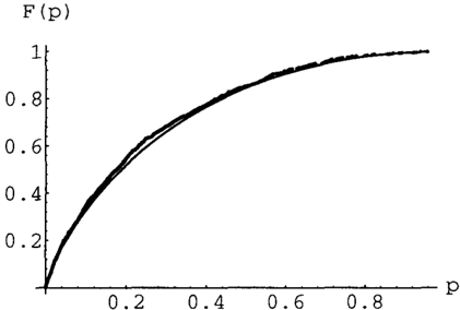
The quality of the estimator (10) is illustrated in Fig­ ure 7, where the scatter plot of the estimated G(p) and the exact G(p) are shown.

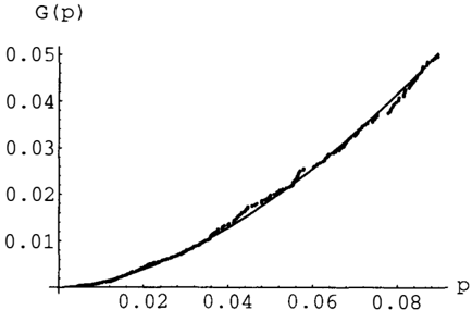
We have selected a threshold value u = 0.0951, which corresponds to 0.05% of the total probability, and we have estimated 8 and a using the Algorithm II. The obtained estimated are 8 = 0.0936 and & = 0.625. Figure 8 shows the sample and the estimated model

p

values, showing a good fitting. Finally, Figure 9 shows the exact and the estimated models for G(p).

Table 1 shows the exact F(p) and G(p), and the esti­ mated G(p) for different values of p.

Note that we used a Bayesian belief network with a few nodes only to be able to perform exact evaluation. However, there is just one random variable P involved in the presented theory. So, the required sample size does not depend on the size of the network.

p	F(p)	G(p)	G(p)
0.05	0.1998	0.0174	0.0176
0.01	0.0561	0.00102	0.00109
0.005	0.0315	0.000289	0.000268
0.002	0.0144	0.0000537	0.0000136

Table 1: Exact, F(p) and G(p) and estimated G(p) for different values of p.

6 CONCLUSIONS

We presented a method for estimating the total con­ tribution G( q) of the events with probability smaller than q to the marginals based on extreme value theory. The estimate of G( q) can be used in various techniques involving Bayesian belief networks: the number of iter­ ations for some simulation algorithms (3, 4] can be cal­ culated such that a certain error bound is guaranteed; the number of assignments in discrete approximation algorithms [5, 15] can be determined; a reasonable size of a cache [14] for storing cases can be computed.

Our theory is applicable to Bayesian belief networks with discrete, or continuous variables. The presented theory can easily be extended for belief networks with mixed discrete, and continuous variables. Experimen­ tal results suggest that our model gives a good approx­ imation of G. However, the log-normal approximation proposed by Druzdzel [12] is inapplicable for estimat­ ing G.

It would be interesting to investigate techniques for in-

crementally updating G when evidence is observed. If only discrete variables are involved, each instantiation can be stored together with case in the sample used for estimating G. When evidence is entered into the belief network, those cases in the sample that are not con­ form the observed evidence can be replaced by new to be generated cases. The other cases can stay unaltered in the sample, thus saving a lot of computational ef­ fort. Experiments have to be performed to get insight in how well the obtained sample is representative for G.

APPENDIX: PROOF OF THEOREM

In this appendix we proof Theorem 2. Assume, with­ out loss of generality that i < j, which implies Pi :S Pj and Ci ::; Cj < 0, and consider the following function of 8,

which is defined in the set { ( -oo, 0) U ( u - Pi, oo )}. Then, Equation (14) can be written as

that is, the solutions of (14) are the zeroes of (26). Clearly, two zeroes of h(8) are 8 = ±oo. We now show that there exist a finite solution of (27).

The function h(8) has the following properties:

Additionally, it has no relative maximum and only one relative minimum which is given by

The solutions of (29) are 80 = ±oo and

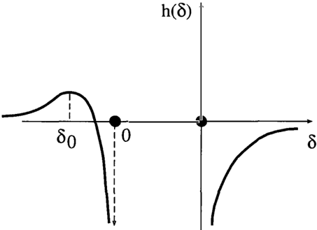
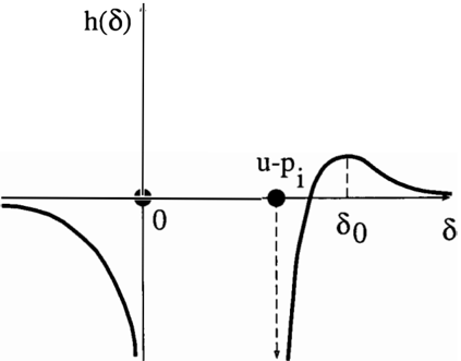
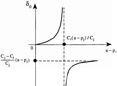
Thus, we have, see Figure 10,

The continuity of h(8) together with (28) and the exis­ tence of a relative minimum, imply that h(8) has only one finite zero if Cj(u- pi)-/= Ci(u-pj)· This zero is in the interval ( u-Pi, 8o) if Ci(u-Pj)-Cj (u-Pi) <= 0, see Figure 11, or in the interval (8o,O) if Ci(u - Pj)­ Cj(u-Pi) > 0, see Figure 12. Thus, we can use the bisection method to determine the solution of (14) (or the zero of h( 8)). This completes the proof.

Acknowledgements

The authors are grateful to the Direcci6n General de Investigaci6n Cientffica y Tecnica (DGICYT) (project PB92- 0504), for partial support of this work. The second author likes to express his thanks to Enrique Castillo and Jose Manuel Gutierrez for inviting him to the University of Cantabria.

References

1. B.C. Arnold. A Class of Hyperbolic Lorenz Curves Sankhya, B, volume 48, pages 427-436, 1986.
2. B.C. Arnold and C. A. Robertson and P. L. Brock­ ett and B.Y. Shu. Generating Ordered Families of Lorenz Curves by Strongly Unimodal Distribu­ tions. Journal of Business and Economic Statis­ tics, volume 5, pages 305-308, 1987.

Fi g ure 12: Plot of h(8) versus 8 for the case u- Pi > Ci(u- Pn)/Ci.

1. R.R. Bouckaert. A stratified simulation scheme for inference in Bayesian belief networks. In Pro­ ceedings Uncertainty in Artificial Intelligence, vol­ ume 10, pages 111-117. Morgan Kaufmann, 1994.
2. ( 4] R.R. Bouckaert, E. Castillo, and J.M. Gutierrez. A modified simulation scheme for inference in Bayesian networks. Under review, 1994.
3. R.R. Bouckaert, E. Castillo, and Gutierrez J.M. A simulation scheme with probability error control for inference in Bayesian networks. Under review, 1994.
4. E. Castillo. Extreme value theory in Engineering. Academic Press, New York, 1988.
5. E. Castillo and A. Hadi. A method for estimating parameters and quantiles of distributions of contin­ uous random variables. Computational Statistics and Data Analysis, volume 9, 1995.
6. E. Castillo and A. Hadi. Estimation in the gener­ alized Pareto distribution. Under review, 90, 1995.
7. E. Castillo and A. Hadi. Parameter and quantile estimation for the generalized extreme-value distri­ bution. Environmetrics, volume 5, pages 417-432. Wiley, 1994.
8. D. Chotikapanich. Comparison of Alternative Functional Forms for the Lorenz Curve. Economics Letters, volume 41, pages 129-138, 1993.
9. J. L. Gastwirth. A General Definition of the Lorenz Curve. Econometrica, volume 39, pages 1037-1039, 1971.
10. M. Druzdzel. Some properties of joint probability distributions. In Proceedings Uncertainty in Arti­ ficial Intelligence, volume 10, pages 187-194, 1994.
11. M. Henrion. Propagating uncertainty in Bayesian networks by probabilistic logic sampling. In Pro­ ceedings Uncertainty in Artificial Intelligence, vol­ ume 4, pages 149-163. North-Holland, 1988.
12. E. Herskovits and G.F. Cooper. Algorithms for Bayesian belief-network precomputation. Methods of Information in Medicine, 30:81-89, 1991.
13. Eugene Santos Jr. and Solomon Eyal Shimony. Belief updating by enumerating high-probability independence-based assignments. In Proceedings Uncertainty in Artificial Intelligence, volume 10, pages 506-513. Morgan Kaufmann, 1994.
14. Uffe Kjrerulff. Reduction of computational com­ plexity in Bayesian networks through removal of weak dependences. In Proceedings Uncertainty in Artificial Intelligence, volume 10, pages 374-382. Morgan Kaufmann, 1994.
15. J. Pearl. Probabilistic Reasoning in Intelligent Systems: Networks of Plausible Inference. Morgan Kaufmann, San Mateo ( CA ) , 1988.
16. J. Pickands. Statistical Inference Using Extreme Order Statistics. In The Annals of Statistics, vol­ ume 3, pages 119-131, 1975.
17. P. J. Rousseeuw, Least Median of Squares Re­ gression. In Journal of the American Statistical Association, volume 79, pages 871-880. Morgan Kaufmann, 1994.
18. P. J. Rousseeuw and A. M. Leroy. Robust Regres­ sion and Outlier Detection. John Wiley and Sons, 1987.