Evaluating Influence Diagrams using LIMIDs

Dennis Nilsson Steffen L. Lauritzen

Department of Mathematical Sciences Aalborg University Fredrik Bajers Vej 7E 9220 Aalborg Denmark

Abstract

We present a new approach to the solu­ tion of decision problems formulated as in­ fluence diagrams. The approach converts the influence diagram into a simpler structure, the Limited Memory Influence Diagram (LIMID), where only the requisite informa­ tion for the computation of optimal policies is depicted. Because the requisite information is explicitly represented in the diagram, the evaluation procedure can take advantage of it. In this paper we show how to convert an influence diagram to a LIMID and describe the procedure for finding an optimal strategy. Our approach can yield significant savings of memory and computational time when com­ pared to traditional methods.

1 INTRODUCTION

Influence Diagrams (IDs) were introduced by Howard and Matheson (1981) as a compact representation of decision problems. Since then, various authors have attempted to formalize their approach and develop al­ gorithms for evaluating IDs.

Olmsted (1983) and Shachter (1986) initiated research in this direction. Their methods operate directly on the ID and consist of eliminating nodes from the di­ agram through a series of value preserving transfor­ mations. During the transformations the policies for the decisions are computed. Later Shachter and Ndi­ likilikesha (1993) and Ndilikilikesha (1994) proposed a similar, but more efficient approach.

Other algorithms evaluate IDs by converting them into different structures. Cooper (1988) described an ap­ proach where the evaluation of IDs is transformed into inference problems for Bayesian networks. Several im­ provements of this method were later proposed by

Shachter and Peot (1992) and Zhang (1998). Shenoy (1992) presented a method where the ID is converted into a valuation network, and the optimal strategy is computed through the removal of nodes from this dia­ gram by fusing the valuations bearing on the node to be removed. Jensen et al. (1994) compiled the ID into a secondary structure, the strong junction tree, and solved the decision problem by the passage of messages towards the root of the tree.

Our work relies on a property that has already been stressed by Shachter (1998, 1999), and Nielsen and Jensen (1999). Namely that in decision problems rep­ resented as IDs there may be information which is not requisite for computing the policies. Going further, we transform the ID into a similar, but simpler, structure termed Limited Memory Influence Diagram (LIMID) where the requisite information is explicitly depicted, and present a simple algorithm for finding the opti­ mal strategy using this reduced structure. This can result in significant gains in efficiency compared to tra­ ditional methods for solving IDs.

Section 2 gives a basic description of LIMIDs as de­ veloped in Lauritzen and Nilsson (1999). For proofs not given in the present paper, the reader is referred to this source.

2 LIMIDS

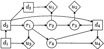
LIMIDs are represented by directed acyclic graphs (DAGs) with three types of nodes. Chance nodes, shown as circles, represent random variables. Decision nodes, shown as squares, represent choices or actions available to the decision maker. Finally, value nodes, shown as diamonds, represent local utility functions. The arcs in a LIMID have a different meaning based on their target. Arcs pointing to utility or chance nodes represent probabilistic or functional dependence. Arcs into decision nodes indicate which variables are known to the decision maker at the time of decision. Thus they in particular imply time precedence.

In contrast with traditional IDs, the LIMID can repre­ sent decision problems that violates the assumption of no forgetting saying that variables known at the time of one decision must also be known when all later de­ cisions are made.

The following fictitious decision problem borrowed from Lauritzen and Nilsson (1999) illustrates a typical decision situation which is well described by a LIMID.

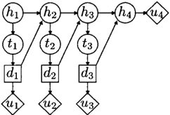
A pig breeder is growing pigs for a pe­ riod of four months and subsequently selling them. During this period the pig may or may not develop a certain disease. If the pig has the disease at the time when it must be sold, the pig must be sold for slaughtering. On the other hand, if it is disease free, its expected market price as a breeding animal is higher. Once a month, a veterinary doctor sees the pig and makes a test for presence of the dis­ ease. The test result is not fully reliable and will only reveal the true condition (hi) of the pig with a certain probability. Based on the test result (ti), the doctor decides whether treating the pig for the disease ( di).

The diagram above represents the LIMID correspond­ ing to the situation where the pig breeder does not keep individual records for his pigs and has to make his decision knowing only the given test result. The memory has been limited to the extreme of only re­ membering the present. In the LIMID, the util­ ity nodes u1, u2, u3 represent the potential treatment costs, whereas u4 is the (expected) market price of the pig as determined by its health at the fourth month.

2.1 SPECIFICATION OF LIMIDS

Suppose we are given a LIMID C with decision nodes 6. and chance nodes r. We let V = 6. U r. The set of value nodes is denoted Y.

For a node n we let pa(n) denote its parents. Each node n E V is associated with a variable which we likewise denote by n, that takes a value in a finite set Xn. For W � V we write Xw = XnEWXn. Typical elements in Xw are denoted by lower case values such as xw, abbreviating xv to x.

Associated with every chance node r (connoting random variable) is a non-negative function Pr on Xr X Xpa(r) such that

where the sum is over Xr. The term Pr does not in general correspond to a true conditional distribution but rather a family of probability distributions for r parametrized by the states of pa(r).

Each value node u E Y is associated with a real func­ tion Uu defined on Xpa(u).

2.2 POLICIES AND STRATEGIES

A policy for decision node d can be regarded as a pre­ scription of alternatives in xd for each possible obser­ vation in Xpa(d). To allow for the possibility of ran­ domizing between alternatives, we formally define a policy as follows. A policy Jd for d is a non-negative function on xd X Xpa(d) which indicates a probabil­ ity distribution over alternative choices for each pos­ sible value of pa( d). They must also satisfy the rela­ tion ( 1) as above. A strategy is a collection of policies { Jd : d E 6.}, one for each decision.

A strategy q = { Jd : d E 6.} determines a joint distri­ bution of all the variables in V as

and Pr and Jd are indeed true conditional distributions w.r.t. fq·

The expected utility of the strategy q is given by

where U = �uEY Uu is the total utility. We are searching for an optimal strategy ij satisfying

Such an optimal strategy is termed a global maximum strategy in Lauritzen and Nilsson (1999).

2.3 SOLUBLE LIMIDS

The complexity of finding optimal strategies within LIMIDs is in general prohibitive. This task, however, becomes feasible for LIMIDs that have a certain struc­ ture. For that reason they are termed soluble. In this section we formally define soluble LIMIDs and present a simple and efficient algorithm for evaluating them.

For a strategy q = { Jd : d E 6.} and any do E 6. we let

be the partially specified strategy obtained by retract­ ing the policy at do.

A local maximum policy for a strategy q at d0, is a policy J�0 which satisfies

So, J�0 is a local maximum policy for q at do if and only if the expected utility does not increase by changing the policy J�0 given the other policies are as in q. The following lemma gives a method to find a local maxi­ mum policy. Here, f q _ d is defined through (2) and the partial strategy obtained from q by retracting Jd. Let­ ting the family of n be defined by fa( n) = pa( n) U { n} we now have

Lemma 1 A policy Jd is a local maximum policy for a strategy q at d if and only if for all Xfa(d) with Jd(xd I Xpa(d)) > 0 we have

As we shall see in Theorem 1, an important instance of Lemma 1 is when the strategy q is the uniform strategy . Here the uniform strategy ij is defined as the strategy ij = {Jd: d E �}, where

Letting

we now have the following special case of Lemma 1.

Corollary 1 A policy Jd is a local maximum policy for the uniform strategy at d if and only if for all Xfa(d) with Jd(xd I Xpa(d)) > 0 we have

Proof: For the uniform strategy ij we have from (2) and (3) that f il -d ex f. Now the corollary follows from Lemma 1. ·

An optimum policy for do in the LIMID £ is a policy which is a local maximum policy at d0 for all strategies q in £. Evidently some decision nodes may not have an optimum policy. However, in the following we present a method for (graphically) identifying decision nodes that have an optimum policy. For this purpose we let the symbolic expression

denote that A and Bare d-separated by Sin the DAG formed by all the nodes in the LIMID £, i.e. including the utility nodes.

For a node n we let de(n) denote the descendants of n. We say that a decision node do is extremal in the LIMID £ if

for every utility node u E de ( d0 ).

Theorem 1 establishes the connection between opti­ mum policies and extremal decision nodes.

Theorem 1 If decision node d is extremal in the LIMID £, then

• d has an optimum policy ;
• any local maximum policy for the uniform strategy at d is an optimum policy for d.

Suppose decision node d is extremal in the LIMID £. Then Theorem 1 ensures that d has an optimum pol­ icy Jd. We can now implement Jd by converting d into a chance node with Jd as the associated conditional probability distribution to obtain a new LIMID £*. It is easily seen that every optimal strategy q* for £* then generates an optimal strategy for £ as q = q· U { Jd } · Thus, if £* again has an extremal decision node, we can yet again find an optimum policy and convert £* as above. If the process can continue until all deci­ sion nodes have become chance nodes, we have clearly obtained an optimal strategy for £.

We thus define an exact solution ordering d1, ... , dk of the decision nodes in £ as an ordering with the prop­ erty that for all i, di is extremal in the LIMID where di+l, . .. , dk have been converted into chance nodes. A LIMID £ is said to be soluble if it admits an exact solution ordering.

Accordingly, computing an optimal strategy for a sol­ uble LIMID £ can be done using the following routine:

Algorithm SINGLE POLICY UPDATING

Input: A soluble LIMID £ with exact solution order­ ing d1 , ... , dk.

For i = k, . . . , 1 do:

1. Compute an optimum policy Jd; for di;
2. Convert di into a chance node with Jd; as its associated conditional probability function.

Return: The policies { Jdk,

... , Jd 1 }.

Note that the policy Jd; computed in step 1 is only optimum for di in the LIMID where decision nodes di+1, ... , dk are converted into chance nodes. The al­ gorithm is well-defined since, as described above, the solubility of £ guarantees that it is always possible to compute an optimum policy for di in step 1. Thus the collection { Jdk, ... , Jd1} constitutes an optimal strat­ egy for £.

3 EVALUATING INFLUENCE DIAGRAMS USING LIMIDS

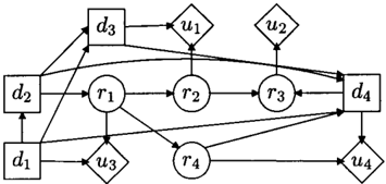
Suppose we are given a decision problem represented by an ID and wish to evaluate it using the algorithm SINGLE POLICY UPDATING. Then one first needs to transform the ID into an 'equivalent' LIMID. This is an easy task: The ID requires a linear temporal order on the decision nodes and, in addition it assumes 'no forgetting', i.e. all variables known at the time of one decision are assumed to be known when subsequent decisions are made. Thus, for an ID with decision nodes d1, ... , dk (where their index indicate the order of the decisions), the no forgetting assumption can be made explicit by drawing arcs from fa( dj) into di for all i and for all j < i. We call the diagram produced in this way the LIMID version of the ID. In Fig. 1-2, an ID and its LIMID version are shown. Now we have

Theorem 2 The LIMID version of an ID is soluble .

Proof: Suppose we are given an ID with decision nodes d1, ... , dk. For the LIMID version £ of the ID we have

for all i, so di is clearly extremal after making di+1, ... , dk into chance nodes. Thus £ is soluble with exact solution ordering d1, ... , dk. ·

3.1 REDUCING SOLUBLE LIMIDS

Starting from a soluble LIMID £ we now present a method for identifying parents of decision nodes that are non-requisite for the computation of optimum poli­ cies. Similar methods for IDs have been produced by Nielsen and Jensen (1999) and Shachter (1999) and when a LIMID is representing an ID their mehod iden­ tifies the same requisite parents as ours, but the sub­ sequent use of SINGLE POLICY UPDATING exploits this reduction to obtain lower complexity of the computa­ tions.

As for IDs the key to simplification of computational problems for LIMIDs is the notion of irrelevance as expressed through the notion of d-separation (Pearl

1986). We say that a node n E pa( d ) in £ is non­ requisite for d if

for every utility node u E de( d). If the above condition is not satisfied, then n is said to be requisite for d.

A reduction of £ is a LIMID obtained by successive removals of arcs from non-requisite parents of deci­ sion nodes. It can be shown that any LIMID £ has a unique minimal reduction, denoted Lmin, obtained by reducing £ as much as possible. Thus in Lmin all parents of decision nodes are requisite ( cf. Theorem 4 in Lauritzen and Nilsson (1999)).

Reducing a soluble LIMID to its minimal reduction can be done by applying the following routine. Note that the algorithm runs in time O(k(graph size)).

Algorithm Reducing Soluble LIMIDs

Input: A soluble LIMID with exact solution ordering dl, . . . ' dk.

For i = k, . . . , 1 do: Remove arcs from non-requisite parents of decision node di.

Note that in the above algorithm the decision nodes are visited in the reverse order starting from dk. This ordering is important: If we chose some other order­ ing there is no guarantee that the reduced LIMID is minimal. For a discussion of this issue the reader is referred to Lauritzen and Nilsson (1999).

Fortunately, the maximum expected utility is pre­ served under reduction, i.e. if c ' is a reduction of £, then the optimal strategy in c ' and the optimal strategy in £ have the same expected utility. In addi­ tion, solubility is preserved under reduction, i.e. any reduction of a soluble LIMID £ is itself soluble. The reader interested in the details and proofs is referred the above source; here we shall use the following the­ orem.

Theorem 3 If the L IM ID £ is soluble, then

1. its minimal reduction Lmin is soluble;
2. any optimal strategy for Lmin is an optimal strat­ egy for £.

Example 1 Regard the ID in Fig. 1, and its LIMID version depicted in Fig 2. The latter diagram is the starting point for reducing the decision problem using Procedure 1:

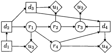
First one notes that u2 and u4 are the only utility nodes that are descendants of d4. Furthermore

so d1 and d3 are non-requisite parents of d4. So the arcs from d1 and d3 into d4 are removed and we let £1 denote the reduced LIMID. Now one notes that in £1, u1 is the only utility node that is a descendant of d3 and since

d1 is non-requisite for d3 and the arc from d1 into d3 is removed. In the reduced LIMID it can be seen that d1 (which is the only parent of d2) is requisite for d2. Finally, d1 has no parents so no further reduction is possible and therefore the reduced LIMID, shown in Fig. 3, is minimal.

3.2 CONSTRUCTION OF JUNCTION TREES

As we shall see, computing optimum policies for the decisions during SINGLE POLICY UPDATING can be done by message passing in a so-called junction tree. In the present section we describe how to compile a soluble LIMID into the junction tree. Clearly it is al­ ways advantageous to start with a minimal LIMID:

Figure 3: The minimal reduction of the LIMID in Fig. 2

while not affecting the correctness of the algorithm, the arcs from non-requisite parents introduce unnec­ essary computations.

The transformation from a LIMID C to a junction tree starts by adding undirected edges between all nodes with a common child (including children that are de­ cision nodes). Then we drop the directions on all arcs and remove all value nodes to obtain the moral graph. Next, edges are added to the moral graph to form a triangulated graph and the cliques are subsequently organized into a junction tree. This can be done in a number of ways; we refer to Cowell et al. (1999) for de­ tails. It is important to note that, in contrast with the local computation method described by Jensen et al. (1994) the triangulation does not need to respect any specific partial ordering of the nodes, but the trian­ gulation can simply be chosen to minimize the com­ putational costs, for example as described in Kjrerulff (1992) 0

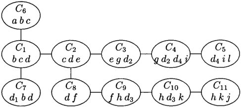
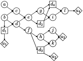
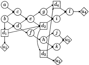
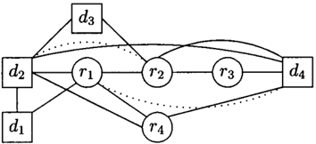
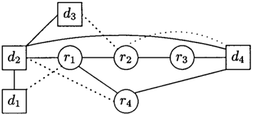
Example 2 Fig. 4 shows the moral graph of the min­ imal LIMID in Fig. 3, and Fig. 5 displays the triangu­ lation of the moral graph. The elimination order used in the triangulation process is chosen to minimize the

Figure 7: The strong junction tree of the original ID represented in Fig. 1. The rightmost clique is the strong root.

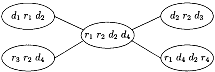
size of the cliques; in particular the ordering does not respect the partial ordering of the nodes in the minimal LIMID. The junction tree for the triangulated graph is given in Fig. 6.

For comparison we have shown the strong junction tree in Fig. 7. Even though the latter has fewer cliques than our junction tree, the largest clique in the strong junction tree contains six variables whereas the largest clique in our junction tree only contains four variables. This is important since the largest clique in the junc­ tion tree mainly determines the complexity of message passing in the junction tree.

3.3 LIMID POTENTIALS

In our junction tree we represent the quantitative el­ ements of a LIMID through entities called LIMID­ potentials, or just potentials for short.

Let W � V. A potential on W is a pair 71W = (pw,uw) where

• pw is a non-negative real function defined on Xw;
• uw is a real function defined on Xw.

So a potential consists of two parts where the first part pw is called the probability part and the second part uw is called the utility part. A potential is called vacuous if its probability part is equal to unity and its utility part is equal to zero. To evaluate the de­ cision problem in terms of potentials we define two basic operations of combination and marginalization. This notion of operations is similar to what is used in Shenoy (1992), Jensen et al. (1994), and Cowell et al. (1999).

The combination of two potentials 1rw 1 = ( P w 1 , uw 1 ) and 1rw2 = (pw2 , u w2), denoted 7rW1 @ 1rw2 , is the potential on wl u w2 given by

The marginalization of the potential 1rw = (pw, uw) onto wl � w' denoted 7fw 1 is the potential on wl given by

Here we have used the convention that 0/0 = 0.

Two potentials 1rw = ( P W, u}v) and 1r� = (p�, u�) are considered equal, and we write 7rW = 1r� if for all xw we have

• p}v(xw) = p�(xw) and
• uw(xw) = u�(xw) whenever p}v(xw) > 0.

This identification of two potentials is needed to prove that marginalization and combination satisfy the ax­ ioms of Shenoy and Shafer (1990) (cf. Lemma 2-4 in Lauritzen and Nilsson (1999)). This in turn estab­ lishes the correctness of the message passing scheme presented in Section 3.5.

3.4 INITIALIZATION

To initialize the junction tree T, one assigns a vacuous potential to each clique C E C. Then for each chance node r in the LIMID C one multiplies the conditional probability function Pr onto the probability part of any clique containing fa(r). When this has been done, one takes each value node u, and adds the local utility function Uu to the utility part of the potential of any clique containing pa( u). The moralization process has ensured the existence of such cliques.

Let 1r c = (pc, uc) be the potential on clique C after initialization. The joint potential 1rv on T is equal to the combination of all potentials and satisfies:

where f is defined in (3) and U is the total utility.

3.5 PASSAGE OF MESSAGES

Let { 1rc : C E C} be a collection of potentials on the junction tree T, and let 1rv = ®{ 1rc : C E C} be the joint potential on T. Suppose we wish to find the marginal 1rt R for some clique R E C. To achieve our purpose we present a propagation scheme where mes­ sages are passed via a mailbox placed on each edge of the junction tree. If the edge connects cl and c2, the mailbox can hold messages in the form of potentials on C1 n C2. So when a message is passed from C1 to C2 or vice versa, the message is inserted into the mailbox.

Imagine for the moment that we direct all the edges in T towards the 'root-clique' R. Then each clique passes a message to its child after having received messages from all its other neighbours. The structure of a mes­ sage 7f C1 -t C2 from clique C1 to its neighbour C2 is given by

where ne(C1) are the neighbours of C1 in T

In words, the message which C1 sends to its neighbour C2 is the combination of all the messages that C1 re­ ceives from its other neighbours together with its own potential, suitably marginalized.

The following result follows from the fact that the two mappings, combination ( Q9) and marginalization (.!.) obey the Shafer-Shenoy axioms.

Theorem 4 Suppose we start with a joint potential 71'V on a junction tree T with cliques C, and pass messages towards a 'root-clique' R as described above. When R has received a message from each of its neigh­ bours ne(R), the combination of all messages with its own potential is equal to the marginalization of 71'V onto R:

3.6 COMPUTING OPTIMUM POLICIES BY MESSAGE PASSING

This section is concerned with showing how to find op­ timum policies for extremal decision nodes by message passing in the junction tree T.

Let 71' W = (Pw, uw) be a potential. The contraction of 'lf'W, denoted cont ( 71'W), is defined as the real function on Xw given by

Accordingly, for the joint potential 71'V defined by (4) we have

It is easily shown that for a potential 'lf' W on W and W1 � W we have

To compute an optimum policy for an extremal deci­ sion node d, one first note that by (5) and (6)

Consequently, an optimum policy for d can be found as follows. First one identifies a clique, say R, that con­ tains fa( d). The compilation of a LIMID £ to a junc­ tion tree T guarantees the existence of such a clique. Then the following steps are carried out ( cf. Corol­ lary 1 and Theorem 1):

1. Collect: Collect to R to obtain 71' R = 71't R as in Theorem 4.
2. 2 Marginalize· Compute 7r* - (7r* ) tfa(d) · ' fa(d) R ·
3. Contract: Compute the contraction Cfa(d) of 7f'f a(d) '
4. Optimize: Define Jd(Xpa(d)) for all Xpa(d) as the distribution degenerate at a point x;'t satisfying ( cf. Corollary 1)

Note that all the computations apart from the second step are local in the root clique R.

Recall that, in SINGLE POLICY UPDATING, when an optimum policy Jd for d has been computed, d is con­ verted into a chance node with Jd as its associated probability function. To make an equivalent conver­ sion in our junction tree, we simply multiply Jd onto the probability part of any clique containing fa(d).

3.7 COMPUTING THE OPTIMAL STRATEGY BY PARTIAL COLLECT PROPAGATIONS

Suppose we have transformed a soluble LIMID £ with exact solution ordering d1, . . . , dk into a junction tree T. The propagation scheme presented here can be used to compute the optimum policies during SINGLE POLICY UPDATING.

As an initial step messages are collected towards any root clique Rk which contains fa(dk)· Then we com­ pute an optimum policy for dk, as described in the previous subsection, and the obtained policy is multi­ plied onto the probability part of Rk.

In a a similar manner the policy for dk_1 can be com­ puted: First, we identify a new root clique Rk-1 which contains fa(dk-d· Then we could collect messages to Rk-1 as above; however, this usually involves a great deal of duplication. Instead we only need to pass mes­ sages along the (unique) path from the old root clique Rk to Rk-1· This is done by first emptying the mail­ boxes on the path and then passing the messages. Note that after this 'partial' collection of messages, Rk-1 has received messages from all its neighbours. Now, an optimum policy for dk-I can be computed and the potential on Rk-I is changed appropriately.

Proceeding in this way by successively collecting mes­ sages to cliques containing the families of the decisions we eventually compute all the optimum policies and thus the optimal strategy.

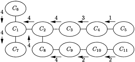
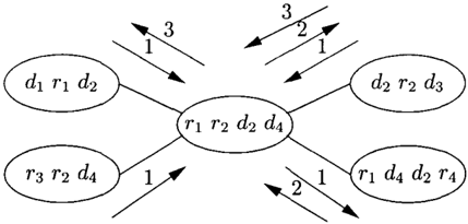
Example 3 Fig. 8 shows how the propagation scheme works on our junction tree. For simplicity of exposition we have omitted the mailboxes in the junction tree.

In our propagation scheme we successively collect messages towards cliques that contain the variables fa(d4), ... ,fa(d1) respectively. So we begin by collect­ ing messages to clique { r1, d4, d2, r 4} since it contains fa(d4) = {d4,r4,d2}. Then we compute an optimum policy for d4 and modify the probability part on the clique by multiplying it with the obtained policy for d4. Now we partial collect messages towards clique {d2,r2,d3} because it contains fa(d3). After comput­ ing an optimum policy for d3 and modifying the poten­ tial appropriately we partial collect messages towards clique {d1,r1,d2}. Note that this clique not only con­ tains fa(d2) but it also contains fa(dl), and thus we need not pass any more messages.

4 REFINEMENT OF THE ALGORITHM

Because multiple collect operations are performed in T, we may pass many messages in the course of the evaluation of all the decisions. In the present section we give a condition for certain collect operations being unnecessary.

Suppose, at some stage in the algorithm, that the pol­ icy for decision d is to be computed, and let R be any clique containing fa(d). In order to compute an optimum policy for d we collect messages towards R. The following theorem states a condition for when a message from a neighbour of R is superfluous.

Theorem 5 Let C be a neighbour of clique R. Then, whenever S = C n R � pa( d), the optimum policy for d can be computed without the message from C.

Proof: Let 7rR = (pR, uR ) be the potential on R after combining it with the messages from all its neighbours except C. Further, suppose S = R n C � pa(d) and let ns = (ps, u s) be the message from C. We need to show that for computation of the optimum policy for d as described in Section 3.6, the message ns is not needed.

Using (6) we have

and

Clearly, asS� pa(d) � fa(d) we have that

where co = Ps 2: 0 depends on Xp a(d) only.

Since f ex fq, where f and /q are given in (2) and (3) we have

where cis a constant. Because

is constant for fixed Xpa(d) , this yields

where c1 depends on Xp a(d) only.

Combining (7) and (8) now yields for fixed Xpa(d)

where c0 2: 0, i.e. for each fixed Xp a(d) , the quantities to be optimized with and without the message from R are linearly and positively related. This completes the proof. ·

The following example shows an application of Theo­ rem 5.

Example 4 The ID displayed in Fig. 9 was intro­ duced by Jensen et al. (1994). Fig. 10 shows the min­ imal reduction of the LIMID version of the ID and Fig. 11 shows the junction tree of the minimal reduc­ tion.

In order to compute the optimum policy for d4 we collect flows towards clique c4 since c4 contains fa(d4)·

However, an application of Theorem 5 gives that the message from c3 is unneccessary: c3 n c4 is a subset of pa(d4) in the minimal reduction in Fig. 10. Thus, we will only need the message from C5. Furthermore, to compute the optimum policy for d3 we collect flows towards clique C9 since it contains fa(d3). But the flow from C8 to C9 is unnecessary because Cs n Cg is contained in pa(d3). Thus, only the flow from Cw to C9 is needed because it has not been computed earlier.

Continuing in this way, it turns out that only one flow along every edge in T is needed for the evaluation of the decision problem (see Fig. 12). So, by applying Theorem 5 we only need to pass 10 flows which is half the flows we would have passed using the partial prop­ agation scheme presented earlier.

5 DISCUSSION

The method presented here transforms decision prob­ lems formulated as IDs into simpler structures, termed minimal LIMIDs, having the property that all requi­ site information for the computation of the optimal strategy is explicitly represented. It uses recursion to solve the decision problem by exploiting that the en­ tire decision problem can be partitioned into a number of smaller decision problems each of which having one decision node only. A one-off process of compilation

is then performed on the LIMID to produce a higher level graphical structure, the junction tree, that is par­ ticular well suited for efficient evaluation of each of the small decision problems.

The use of recursion is inspired by the well-known trick of Cooper ( 1988) and differs from methods in e.g. Shenoy (1992), and Jensen et al. (1994). By using recursion we do not require the storage of potentially large tables of intermediate results (see for instance Example 2).

As a consequence, our junction tree can always be made as small as the strong junction tree (Jensen et al. 1994), and in some cases our method can result in considerable reduction of evaluation time and mem­ ory. This reduction happens at two levels. At the first level, we obtain a smaller junction tree because we work in the reduced structure that only includes requisite information. At the second level, we obtain a smaller junction tree because we can triangulate the structure obtained without obeying order constraints.

On the other hand, our method typically passes more messages than the strong junction tree method, partly because our junction tree have more (and smaller) cliques, partly because we perform several collect prop­ agations. As the size of the maximal clique most often is crucial for the efficiency of local computation algo­ rithms, our algorithm should generally be fast com-

pared to traditional algorithms.

There are many opportunities to refine and extend this research. In particular it should be possible to reduce the number of messages that are passed in the junc­ tion tree. We have presented one such condition for a message being redundant, but a deeper insight in the partial propagation algorithm may reveal other redun­ dant computations, and improve the efficiency of the algorithm. The new method presented here also opens the possibility of evaluating large and computationally prohibitive decision problems by approximating them with soluble LIMIDs. Work regarding this issue is de­ scribed in Lauritzen and Nilsson (1999) and is still in progress.

Acknowledgements

This research was supported by DINA (Danish Infor­ matics Network in the Agricultural Sciences), funded by the Danish Research Councils through their PIFT programme.

References

• Cooper, G. F. (1988). A method for using belief networks as influence diagrams. In Proceedings of the 4th Work­ shop on Uncertainty in Artificial Intelligence, pp. 5563. Minneapolis, MN.
• Cowell, R. G., Dawid, A. P., Lauritzen, S. L., and Spiegel­ halter, D. J. (1999). Probabilistic Networks and Expert Systems. Springer-Verlag, New York.
• Howard, R. and Matheson, J. (1981). Influence diagrams. In The Principle and Applications of Decision Anal­ ysis, (ed. R. Howard and J. Matheson), pp. 719-62. Strategic Decisions Group, Menlo Park, Calif.
• Jensen, F., Jensen, F. V., and Dittmer, S. L. (1994). From influence diagrams to junction trees. In Proceedings of the 1Oth Conference on Uncertainty in Artificial Intel­ ligence, (ed. R. L. de Mantaras and D. Poole), pp. 36773. Morgan Kaufmann Publishers, San Francisco, CA.
• Kj<Erulff, U. (1992). Optimal decomposition of probabilis­ tic networks by simulated annealing. Statistics and Computing, 2, 19-24.
• Lauritzen, S. L. and Nilsson, D. (1999). LIMIDs of deci­ sion problems. Research Report R-99-2024, Dept. of Mathematical Sciences, Aalborg University. Submit­ ted to Management Science.
• Ndilikilikesha, P. (1994). Potential influence diagrams. International Journal of Approximate Reasoning, 10, 251-85.
• Nielsen, T. D. and Jensen, F. V. (1999). Welldefined de­ cision scenarios. In Proceedings of the 15th Annual Conference on Uncertainty in Artificial Intelligence, (ed. K. Laskey and H. Prade), pp. 502-11. Morgan Kaufmann Publishers, San Francisco, CA.
• Olmsted, S. (1983). On Representing and Solving Decision Problems. PhD thesis, Stanford University.
• Pearl, J. (1986). Fusion, propagation and structuring in belief networks. Artificial Intelligence, 29, 241-88.
• Shachter, R. (1986). Evaluating influence diagrams. Oper­ ations Research, 34, 871-82.
• Shachter, R. (1998). Bayes-ball: The rational pasttime (for determining irrelevance and requisite information in belief networks and influence diagrams). In Proceed­ ings of the Fourteenth Annual Conference on Uncer­ tainty in Artificial Intelligence {UAI-g8), pp. 48-487. Morgan Kaufmann Publishers, San Francisco, CA.
• Shachter, R. ( 1999). Efficient value of information com­ putation. In Proceedings of the 15th Annual Con­ ference on Uncertainty in Artificial Intelligence, (ed. K. Laskey and H. Prade), pp. 594-601. Morgan Kauf­ mann Publishers, San Francisco, CA.
• Shachter, R. and Ndilikilikesha, P. (1993). Using influence diagrams for probabilistic inference and decision mak­ ing. In Proceedings of the Ninth Conference on Uncer­ tainty in Artificial Intelligence, (ed. D. Heckermann and A. Mamdani), pp. 276-83. Morgan Kaufmann, Stanford, California.
• Shachter, R. and Peot, M. A. (1992). Decision making using probabilistic inference methods. In Proceedings of the Eighth Annual Conference on Uncertainty in Artificial Intelligence (UAI-92), pp. 276-83. Morgan Kaufmann Publishers, San Francisco, CA.
• Shenoy, P. P. (1992). Valuation-based systems for Bayesian decision analysis. Operations Research, 40, 463-84.
• Shenoy, P. P. and Shafer, G. R. (1990). Axioms for proba­ bility and belief-function propagation. In Uncertainty in Artificial Intelligence IV, (ed. R. D. Shachter, T. S. Levitt, L. N. Kana!, and J. F. Lemmer), pp. 169-98. North-Holland, Amsterdam.
• Zhang, N. L. (1998). Probabilistic inference in influence di­ agrams. In Proceedings of the Fourteenth Annual Con­ ference on Uncertainty in Artificial Intelligence (UAI98), pp. 514-22. Morgan Kaufmann Publishers, San Francisco, CA.