Evaluating Las Vegas Algorithms Pitfalls and Remedies

H o l g e r H. Hoos and Thomas Stiitzle Computer Science Department Darmstadt University of Technology D-62483 Darmstadt, Germany {hoos,stuetzle}@informatik.tu-darmstadt.de

Abstract

Stochastic search algorithms are among the most sucessful approaches for solving hard combinato­ rial problems. A large class of stochastic search approaches can be cast into the framework of Las Vegas Algorithms (LVAs). As the run-time be­ havior of LV As is characterized by random vari­ ables, the detailed knowledge of run-time distri­ butions provides important information for the analysis of these algorithms. In this paper we propose a novel methodology for evaluating the performance of LVAs, based on the identification of empirical run-time distributions. We exem­ plify our approach by applying it to Stochastic Local Search (SLS) algorithms for the satisfia­ bility problem (SAT) in propositional logic. We point out pitfalls arising from the use of improper empirical methods and discuss the benefits of the proposed methodology for evaluating and com­ paring LV As.

1 INTRODUCTION

Las Vegas algorithms are nondeterministic algorithms with the following properties: If a solution is returned, it is guar­ anteed to be correct, and the run-time is characterized by a random variable. Las Vegas algorithms are prominent not only in the field of Artificial Intelligence but also in other areas of computer science and Operations Research. In the recent years stochastic local search (SLS) algorithms such as Simulated Annealing, Tabu Search, and Evolutionary Al­ gorithms have been found to be very successful for solving NP-hard problems from a broad range of domains. But also a number of systematic search methods, like some modern variants of the Davis Putnam algorithm for propositional satisfiability (SAT) problems, or backtracking-style algo­ rithms for CSPs and graph coloring problems make use of non-deterministic decisions (like randomized tie-breaking rules) and can thus be characterized as Las Vegas algo­ rithms.

Due to their non-deterministic nature, the behavior of Las Vegas algorithms is usually difficult to analyze. Even in the cases where theoretical results do exist, their practical ap- plicability is often very limited, as in the case of Simulated Annealing, which is proven to converge towards an optimal solution under certain conditions which, however, cannot be met in practice. Given this situation, in most cases analyses of the run-time behavior of Las Vegas algorithms are based on empirical methodology. In a sense, despite dealing with completely specified algorithms which can be easily under­ stood on a step-by-step execution basis, computer scientists are in the same situation as, say, an experimental physicist observing some non-deterministic quantum phenomenon.

The methods that have been applied for the analysis of Las Vegas algorithms in AI, however, are rather simplis­ tic. Nevertheless, at the first glance, these methods seem to be admissible, especially since the results are usually quite consistent in a certain sense. In case of SLS algorithms for SAT, for instance, advanced algorithms like WSAT (Selman et a!., 1994) usually outperfonn older algorithms (such as GSAT (Selman et al., 1992)) on a large number of problems from both randomized distributions and structured domains. The claims which are supported by empirical evidence are usually relatively simple (like "algorithm A outperforms al­ gorithm B"), and the analytical methodology used is both easy to apply and powerful enough to get the desired results.

Or is it really? Recently, there has been some severe criti­ cism regarding the empirical testing of algorithms (Hooker, 1994; Hooker, 1996; McGeoch, 1996). It has been pointed out that the empirical methodology that is used to evaluate and compare algorithms does not reflect the standards which have been established in other empirical sciences. Also, it was argued that the empirical analysis of algorithms should not remain at the stage of collecting data, but should rather attempt to formulate hypotheses based on this data which, in turn, can be experimentally verified or refuted. Up to now, most work dealing with the empirical analysis of Las Vegas algorithms in AI has not lived up to these demands. Instead, recent studies still use basically the same methods that have been around for years, often investing tremendous compu­ tational effort in doing large scale experiments (Parkes and Walser, 1996) in order to ensure that the basic descriptive statistics are sufficiently stable. At the same time more fun­ damental issues, such as the question whether the particu­ lar type of statistical analysis that is done (usually estimat­ ing means and standard deviations) is adequate for the type of evaluation that is intended, are often neglected or not ad-

dressed at all.

In this work, we approach the issue of empirical methodol­ ogy for evaluating Las Vegas algorithms for decision prob­ lems, like SAT or CSP, in the following way. After dis­ cussing fundamental properties of Las Vegas algorithms and different application scenarios, we present a novel kind of analysis based on estimating the run-time distributions for single instances. We motivate why this method is superior to established procedures while generally not causing ad­ ditional computational overhead. We then point out some pitfalls of improperly chosen empirical methodology, and show how our approach avoids these while additionally of­ fering a number of benefits regarding the analysis of indi­ vidual algorithms, comparative studies, the optimization of critical parameters, and parallelization.

2 LAS VEGAS ALGORITHMS AND APPLICATION SCENARIOS

An algorithm A is a Las Vegas algorithm for problem class TI, if (i) whenever for a given problem instance 1r E TI it returns a solution s, s is guaranteed to be a valid solution of 11" , and (ii) on each given instance 11", the run-time of A is a random variable RT A , 11"· According to this definition, Las Vegas algorithms are always correct, while they are not necessarily complete. Since completeness is an important theoretical concept for the study of algorithms, we classify Las Vegas algorithms into the following three categories:

• complete Las Vegas algorithms can be guaranteed to solve each soluble problem instance within run-time tmax. where tmax is an instance-dependent constant. Let P(RT A,11" � t) denote the probability that A finds a solution for a soluble instance 1r in time � t, then A is complete exactly if for each 1r there exists some tmax such that P(RT A, 11" � tmax) = 1.
• approximately complete Las Vegas algorithms solve each soluble problem instance with a probability con­ verging to 1 as the run-time approaches oo. Thus, A is approximately complete, if f or each soluble instance 11" , limt-+oo P(RT A , 11" � t) = 1.
• essentially incomplete Las Vegas algorithms are Las Vegas algorithms which are not approximately com­ plete (and therefore also not complete).

Examples for complete Las Vegas algorithms in AI are ran­ domized systematic search methods like modern Davis Put­ nam variants (Crawford and Auton, 1996). Many of the most prominent stochastic local search methods, like Sim­ ulated Annealing or GSAT with Random Walk, are approx­ imately complete, while others, such as basic GSAT (with­ out restart) and most variants of Tabu Search are essentially incomplete.

In literature, approximate completeness is often referred to as convergence. Convergence results an: established for a number of SLS algorithms, such as Simulated Anneal­ ing. Approximate completeness can be enforced for most SLS algorithms by providing a restart mechanism, as can be found in GSAT (Selman et al., 1992). However, both forms of approximate completeness are mainly of theoretical in­ terest, since the time limits for finding solutions are usually far too large to be of practical use.

APPLICATION SCENARIOS

Before even starting to evaluate any algorithm, it is crucial to find the right evaluation criteria. Especially for Las Ve­ gas algorithms there are fundamentally different criteria for evaluation, depending on the characteristics of the environ­ ment they are supposed to work in. Thus, we classify pos­ sible application scenarios in the following way:

• Type 1: There are no time limits, i.e., we can afford to run the algorithm as long as it needs to find a solution. Basically, this scenario is given whenever the computations are done off-line or in a non-realtime environment, where it does not really matter how long we need to find a solution.
• Type 2: There is a time limit tmax for finding a solution. In real-time applications, like robotic control or dynamic scheduling, tmax can be very small.

Type 3: The usefulness or utility of a solution depends on the time needed to find it. Formally, if utilities are repre­ sented as values in (0, 1 ], we can characterize these scenar­ ios by specifying a utility function U : R 1--t [0, 1], where U(t) is the utility of finding a solution after timet. As can be easily seen, types 1 and 2 are special cases of type 3.

Obviously, different criteria are required for evaluating the performance of Las Vegas algorithms in these scenarios. While in the case of no time limits being given (type 1), the mean run-time might suffice to roughly characterize the run-time behavior, in real-time situations (type 2) it is ba­ sically meaningless. An adequate criterion for a type 2 sit­ uation with time-limit tmax is P(RT � tmax), the proba­ bility of finding a solution within the given time-limit. For type 3, the most general scenario, the run-time behavior can only be adequately characterized by the run-time dis­ tribution function rtd : R 1--t (0, 1] defined as rtd(t) = P(RT � t) or some approximation of it. The run-time dis­ tribution (RTD), however, completely and uniquely char­ acterizes the run-time behavior of a Las Vegas algorithm. Given this information, other criteria, like the mean run­ time, its standard deviation, median, percentiles, or success­ probabilities P(RT � t') for arbitrary time-limits t' can be easily obtained.

3 OUR EMPIRICAL METHOD

To answer the questions that arise from the different appli­ cation scenarios discussed in the previous section, it is im­ portant to have knowledge of the actual run-time distribu­ tions (RTD) of Las Vegas algorithms. The run-time is a random variable and we can get knowledge on its distribu­ tion by empirically taking samples of the random variable by simply running the algorithm several times. Based on the sample, assumptions on the type of distribution function can be made. These assumptions can be validated by sta­ tistical hypothesis tests and in case the assumptions cannot be backed up by the sample data, incorrect assumptions are

steps

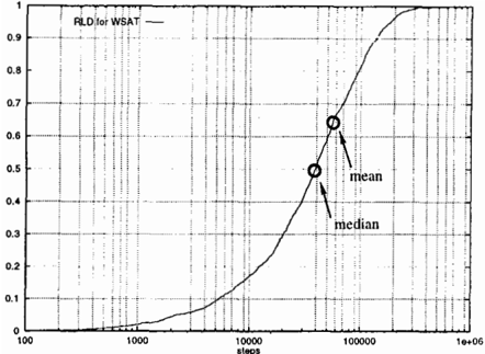
Figure 1: RLD for WSAT on a hard Random-3-SAT in­ stance for optimal parameter settings; median vs. mean.

identified and rejected. As the actual run-time distribution of an Las Vegas algorithm depends on the problem instance, it should be clear that RTDs should be estimated on single problem instances. Yet, this does not limit the type of con­ clusions that may be drawn as general conjectures on the type of run-time distributions over a whole problem class can be formed and tested. We will illustrate this point in more detail in Section 5.1.

Instead of actually measuring run-time distributions in terms of CPU-time, it is often preferable to use represen­ tative operation counts as a more machine independent measure of an algorithm's performance. Using an appro­ priate cost model of the algorithm's operations, operation counts can easily be converted into run-times, facilitating comparisons of algorithms across architectures. Thus, in­ stead of run-time distributions we get run-length distribu­ tions (RLDs). For example, an appropriate operation count for local search algorithms for SAT is the number of local search steps. In the following we will use run-time distribu­ tions and run-length distributions interchangeably as long as they can be converted one into the other.

To actually measure RLDs, one has to take into account that most algorithms have some cutoff parameter like maximum number of iterations, maximum time limit, or others. Prac­ tically, we measure empirical RLDs by running the respec­ tive Las Vegas algorithm for n times on a given problem in­ stance up to some (very high) cutoff value1 and recording for each successful run the number of steps required to find a solution. The empirical run-length distribution is the cumu­ lative distribution associated with the observations. More formally, let rl (j) denote the run length for the jth success­ ful run, then the cumulative empirical RLD is defined by P(rl � i) = l{jlrl(j) � i}lfn. Note, that obtaining run­ length distributions for single instances does not involve a significantly higher computational effort than to get a stable estimate for the mean performance of an algorithm.

To give an example of an actually occuring RLD, we run

1 0ptimal cutoff settings may then be determined a posteriori using the empirical run-time distribution, see Sec. 5.2.

a state-of-the-art local search algorithm (WSAT (Selman et a!., 1994)) on a hard Random-3-SAT instance for optimal walk-parameter settings and present the RLD in Figure 1. The x-axis represents the computational effort as the num­ ber of local search steps, they-axis gives the empirical suc­ cess probability. One may note that the shape of the RLD is that of an exponential distribution ed[m], with distribution function2 F(x) = 12-xfm. Actually, using a x2-test, the hypothesis that the RLD corresponds to an exponential dis­ tribution passed the test. We will discuss potential benefits of our method in more detail in Section 5.

4 PITFALLS OF INADEQUATE METHODOLOGY

4.1 SUPERFICIAL ANALYSIS OF RUN-TIME BEHAVIOR

A well-established method for evaluating the run-time be­ havior of Las Vegas algorithms is to measure average run­ times on single instances in order to obtain an estimate of the mean run-time. Practically, this is done by executing the algorithm n times on a given problem instance with cutoff time tmax· If k of these runs are successful and rt; is the run-time of the ith successful run, the mean run-time is esti­ mated by averaging over the successful runs and accounting for the expected number of runs required to find a solution:

One problem with this method is that the mean alone gives only a very unprecise impression of the run-time behavior, even if additionally the standard deviation (or variance) for the run-time of the successful runs is reported. Consider the design of an algorithm for a type 2 application scenario and the specific question of estimating the cutoff time tmax for solving a given problem instance with a probability p. If only the mean run-time E(RT) is known, the best estimate we can obtain is given by the Markov inequality (Rohatgi, 1976) P(RT 2: t) � E(RT)jt:

If the standard deviation u(RT) is known and finite, using the Tchebichev inequality P(l RT- E(RT) I 2: t: ) � u2(RT)jt:2 we obtain a better estimate:

If, however, we know that the run-time of a given Las Ve­ gas algorithm is exponentially distributed3, we get a much

2 In statistical literature, typically the exponential distribution is presented with respect to base e. With base 2, instead, the advantage is that parameter m corresponds to the median of the distribution.

3 As we will discuss later, assuming an exponential RTD is quite realistic, since we found that this can be observed for a num­ ber of modem stochastic local search algorithms on various prob­ lem classes.

more accurate estimate. In the following example, we see the drastic differences between these three estimates. For a given Las Vegas algorithm applied to some problem the mean run-time and the standard deviation are 100 seconds each, a situation which is not untypical, e.g., for stochas­ tic local search algorithms for SAT. We want to determine the run-time t' required for obtaining a solution probabil­ ity of 0.99. Without any additional knowledge on the run­ time distribution we get an estimate of 1100 sec (using the Tchebichev inequality). If even the standard deviation is un­ known, we can only use the Markov inequality and estimate t' as 10000 sec! But assuming that the run-time is exponen­ tially distributed, we get an estimate of 460 sec. This illus­ trates that as long as the type of RID is not known a pri­ ori, analyzing only means and standard deviations is a very wasteful use of empirical data.

Another problem, especially in recent literature on stochas­ tic local search, lies in the tacit assumption that several pa­ rameters of the considered algorithms can be studied in­ dependently. In specific cases, it is known that this as­ sumption does not hold (Hoos and Stiitzle, 1996; Steinmann et al., 1997). For the evaluation of Las Vegas algorithms in general, it is crucial to be aware of possible parameter de­ pendencies, especially those involving the cutoff time tmax which plays an important role in type 2 and 3 application scenarios.

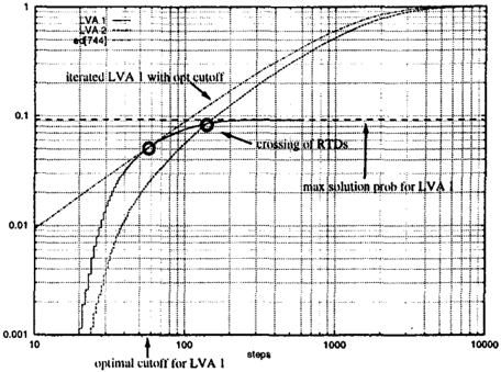
In Fig. 2, we show the RLDs of two different Las Vegas al­ gorithms LVA 1 and LVA 2 for the same problem instance. As can be easily seen, LVA 1 is essentially incomplete with an asymptotic solution probability approaching ca. 0.09, while LVA 2 is approximately complete. Now, note the crossing of the two RLDs at ca. 120 steps. For smaller cutoff times, LVA 1 achieves considerably higher solution probabilities, while for greater cutoff times, LVA 2 shows increasingly superior performance. Actually, using the op­ timal cutoff time of ca. 57 steps in connection with restart, the exponential run-time distribution marked "ed[744]" can be obtained, which realizes a speedup of ca. 24% compared to LVA 2. Thus, the performance of LVA 1 is not only supe­ rior to that of LVA 2 for small cutoff times, but based on the RIDs, it is possible to modify algorithm LVA 1 such that its overall performance dominates that of LVA 2, see also Sec. 5.

As a consequence of these observations, basing the com­ parison of Las Vegas algorithms on expected run times is in the best case unprecise, in the worst case it leads to er­ roneous conclusions. The latter case occurs, when the two corresponding RTDs have at least one intersection. Then, obviously, the outcome of comparing the two algorithms de­ pends entirely on the cutoff time tmax which was chosen for the experiment.

4.2 INHOMOGENEOUS TEST SETS

Often, Las Vegas algorithms are tested on sets of randomly generated problem instances. This method is particularly popular for problem classes, for which phase transition phenomena have been observed, such as Random-3-SAT (Crawford and Auton, 1996) or Random-CSP (Sn:ith and

Dyer, 1996), because instances from the phase-transition re­ gion have been found to be particularly hard. Practically, the test sets for SLS algorithms are usually obtained by gen­ erating a number of sample instances from the phase transi­ tion area and filtering out unsolvable instances using a com­ plete algorithm. The evaluation of Las Vegas algorithms on such a test set is done by evaluating a number of runs on each instance. Usually, the final performance measure is ob­ tained by averaging over all instances from the test set.

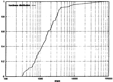
This last step, however, is potentially extremely problem­ atic. Since the run-time behavior on each single instance is characterized by a RID (as discussed above), averag­ ing over the test set is equivalent to averaging over these RIDs. Because in general, averaging over a number of dis­ tributions yields a distribution of a different type, the prac­ tice of averaging over RIDs (and thus the averaging over test sets) is quite prone to producing observations, which do not reflect the behavior of the algorithm on individual instances, but rather a side-effect of this method of evalua­ tion. We exemplify this for Random-3-SAT near the phase­ transition, a problem class which has been used in many studies of stochastic local SAT procedures, such as GSAT or GSAT with random walk (GWSAT) (Selman et al., 1992; Gent and Walsh, 1995). Our own experimental studies have shown, that for GWSAT with optimal walk parameter (as well as for a number of other stochastic local search algo­ rithms, such as WSAT (Selman et al., 1994) or NOVELTY (McAllester et al., 1997)), the RLDs on single instances from this problem distribution can be reasonably well ap­ proximated by exponential distributions (Hoos and Sttitzle, 1998). By measuring the median run-lengths for each prob­ lem instance from a typical randomly generated and filtered test set, we obtain a distribution of the median hardness of the problems as shown in Fig. 3. Since the median run­ lengths were determined using 1000 runs per instance, they are very stable which leaves the random selection of the in­ stances as the main source of noise in the measured distri­ bution.

Since the RLDs for single instances are basically exponen-

-

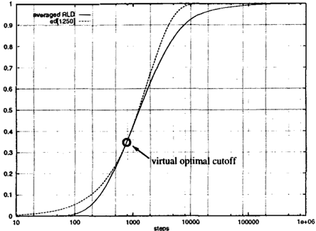
Figure 4: Average RLD for WSAT on the same test s�t. Note the virtual optimal cutoff at ca. 750 steps, for details see text.

tial distributions, optimal cutoff times cannot be observed for individual instances. The reason for this is the fact that for exponential run-time distributions, the probability of finding a solution within k steps of the algorithm is in­ dependent of the number of steps perform _ ed before. (This _ is discussed in more detail in Sec. 5.) Smce the class of exponential distributions is not closed under averag � ng, the combined RLD for all instances in the test set, obtamed by averaging over the individual RLDs, is not exponential � y distributed. But for this combined distribution, shown m Fig. 4, obviously an optimal cutoff time exists, which is ob­ tained by finding the minimal value m* for which _ ed[m*] and the average RLD have at least one common pomt.

Thus while the averaged RLD suggests the existence of an o � erall optimal cutoff time, actually for each single in­ stance, an optimal cutoff time does not exist. Although this might seem a bit paradoxical, this observation can be eas­ ily explained: When averaging over the RLDs, we don't distinguish between the probability of solving different in­ stances. Using the "optimal" cutoff inferred from the av­ erage RLD then simply means that solving some easier in­ stances with a sufficiently high probability compensates for the very small solution probability for the harder instances going along with using this cutoff. Thus, solving easier in­ stances gets priority over solving harder instances. Under this interpretation, the "optimal" cutoff can be considered meaningful. Assuming, however, that in practice the goal in testing Las Vegas algorithms on test sets sampled from random problem distributions is to get a realistic impres­ sion of the overall performance, including hard instances, the "optimal" cutoff inferred from the averaged RLD is sub­ stantially misleading.

The above discussion shows, that by averaging over test sets, generally in the best case one consciously observes a bias for solving certain problems, the practical use of which seems rather questionable. But far more likely, being not aware of these phenomena, the observations thus obtained are misinterpreted and lead to erroneous conclusions. One could, however, imagine a situation in which averaging over test sets is not that critical. This would be given if the test sets are very homogeneous in the sense that the RIDs for each single instance are roughly identical. Unfortunately, this sort of randomized problem distributions seems to be very rare in practice. Certainly, Random-3-SAT is not ho­ mogeneous in this sense, and at least the authors are cur­ rently not aware of any sufficiently complex homogenous randomized problem distribution for SAT or CSP.4

Generally, a fundamental problem with averaging over ran­ dom problem distributions is the mixing of two different sources of randomness in the evaluation of algorithms: the nondeterministic nature of the algorithm itself, and the ran­ dom selection of problem instances. Assuming that in t � e analysis of Las Vegas algorithms one is mostly interested m the properties of the algorithm, at least a very good knowl­ edge of the problem distribution is required for separating the influence of these inherently different types of random­ ness.

5 BENEFITS OF OUR METHOD

5.1 CHARACTERIZING RTDs

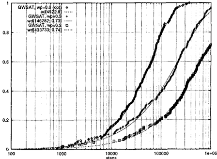
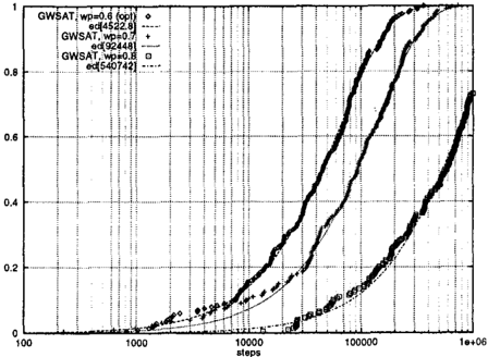
In this section we demonstrate our empirical methodol­ ogy for testing Las Vegas algorithms with stochastic _ local search as one example application and illustrate how mter­ esting observations can be made using our approach. For this purpose we analyze the run-time behavior of GS � T with random walk (GWSAT) on a hard Random-3-SAT In­ stance from the phase transition region using various walk­ probability settings, including the optimal one. The _ walk­ probability wp is, besides the cutoff value, the most Impor­ tant parameter of this algorithm. The algorithm was run 200 times for different settings of wp. Based on the em-

4 There is, however, some indication, that certain randomized classes of SAT encoded problems from other domains, such as compactly encoded subclasses of the Hamilton Circuit Problem (Hoos, 1996), are significantly more homogeneous than Random3-SAT.

steps

steps

Figure 6: Run-time distribution for GSAT with random walk on a hard random 3-SAT instance for optimal and lower-than-optimal walk-parameter settings.

pirical distribution for the optimal noise-parameter setting WPopt we conjectured that the run-time distribution can be well approximated by an exponential distribution. With this hypothesis the parameter m can be estimated and the goodness-of-fit of the empirical distribution can be tested. In our concrete example this hypothesis passed the x2-test.

For larger than optimal noise-parameter settings wp > wp0pt we could verify by the x2-test that the RLDs are ex­ ponentially distributed. Yet, the RIDs are shifted to the right by a constant factor, if using a log-scale on the x-axis as in Figure 5. This means that to guarantee a desired suc­ cess probability, if using wp > WPopt the required number of steps is by a constant factor higher than for wp = wp0pt· A completely different behavior can be observed for wp < WPopt (see Figure 6). In this case, the run-time distribu­ tions cannot be approximated by exponential distributions, but instead we found a good approximation using Weibull distributions wd[m, a ] with F(x) = 12-(x/m)", a < 1. This corresponds to the fact that the higher the desired so­ lution probability, the larger will be the loss of performance w.r.t. the optimal noise setting. Additionally, for instances which are easy to solve we could observe systematic devi­ ations from the distribution assumptions in the lower part. These deviations may be explained by the initial hill-climb phase (Gent and Walsh, 1993), as, intuitively, it needs some time for the algorithm to reach a position in the search space for which there is a realistically high chance of finding a so­ lution.

Our proposed way of measuring and analyzing RTDs shows considerable benefits. The statistical distributions of the RTDs can be identified and the goodness-of-fit can be tested using standard statistical tests. Also, based on such a methodology an experimental approach of testing Las Ve­ gas algorithms along the lines proposed by Hooker (Hooker, 1996) can be undertaken. For example, based on the above discussion one such hypothesis is that for optimal noise pa­ rameter settings for GWSAT, its run-time behavior for the solution of single, hard instances from the crossover region of Random-3-SATcan be well described by exponential dis­ tributions. This hypothesis can be tested by running a se­ ries of experiments on such instances. Doing so, our em­ pirical evidence confirms this conjecture. Similar results have been established for other algorithms, and not only applied to Random-3-SAT but also on SAT-encoded prob­ lems from other domains (Hoos and Sttitzle, 1998). Thus, by studying run-time distributions on single instances, hy­ potheses on the algorithm's behavior on a problem class like random 3-SAT can be formed and tested experimentally. It is important to note that limiting the analysis of RIDs to single instances does not impose limitations on' obtaining and verifying conjectures on the behavior of algorithms on whole problem classes. Furthermore, by measuring RLDs (RIDs) we could observe a qualitatively different behav­ ior of GWSAT, depending on whether lower than optimal or larger than optimal walk-parameter settings are chosen. For wp > wp0pt. the run-time distribution can still be iden­ tified as an exponential distribution, i.e., the type of distri­ bution does not change. On the other hand, if wp < WPopt the type of distribution changes. Based on these observa­ tions further fundamental hypotheses (theories) describing the behavior of this class of algorithms may be formed and experimentally validated.

5.2 COMPARING AND IMPROVING ALGORITHMS

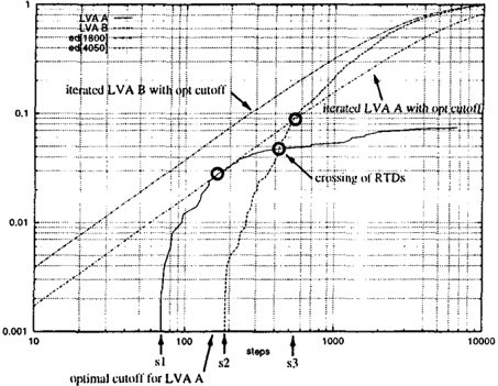
Important aspects like the comparison and design of algo­ rithms can be addressed by the study of RLDs. Consider the situation presented in Figure 7 in which RLDs for two spe­ cific SLS algorithms (LVA A and LVA B) are plotted. LVA B is approximately complete and its performance monoton­ ically improves with increasing run lengths (as can be seen from the decreasing distance between the RLD and the pro­ jected optimal exponential distribution ed[1800]). LVA A is essentially incomplete, the success probability converges to ca. 0.08. For very short runs we also observe "conver­ gent behavior": Apparently for both algorithms there exists a minimal (sample size dependent) number of steps (marked s1 and s 2 on the x-axis) below that the probability to find a solution is negligible. Interestingly, both curves cross in

one specific point at ca. 420 steps; i.e., without using restarts LVA A gives a higher solution probability than LVA B for shorter runs, whereas LVA B is more effective for longer runs. Yet, for LVA A an optimal cutoff value of ca. 170 steps exists. Thus, repeated execution of LVA A for a rea­ sonably well chosen cutoff time, after which the algorithm is restarted, gives a much higher solution probability as ac­ tually observed when running the algorithm for a long time. In fact, if the optimal cutoff parameter is chosen, one more point of interest is at ca. 500 steps (marked 83 on the x-axis): For a lower number of steps as 83, using independent runs of LVA A with optimal cutotf value one improves upon the performance of LVA B, while past 83 LVA B is strictly su­ perior to LVA A. Consequently, an anytime combination of the two algorithms should select LVA A with optimal cu�off up to 83 steps, and then switch to LVA B.

This example illustrates two important points. One con­ cerns the comparison of algorithms. Generally, a Las Ve­ gas algorithm dominates another one, if it consistently gives a higher solution probability. More formally, LVA 1 domi­ nates LVA 2 if for optimal parameter settings \ft : P(RT1 ::; t) 2: P(RT2 ::; t) and 3t : P(RT1 ::; t) > P(RT2 ::; t). In case the RTDs cross over, the comparison of algorithms is substantially more difficult. Then, as detailed in the exam­ ple above, often it occurs that one algorithm is preferable for lower time limits while the other may be better for long run times. In such a case an anytime combination of both algorithm can enhance overall performance.

A further, even more important point concerns the steepness of the run-time distributions. It is well known that for expo­ nentially distributed run-times, due to the properties of the exponential distribution (Rohatgi, 1976), we get the same solution probability running an algorithm once for timet or p times for time tjp. If from some point on the run-tjme distribution of an algorithm is steeper than an exponential distribution, the probability of finding a solution relatively increases when running the algorithm for a longer time. In such a case it would be worse to restart the algorithm after some fixed cutoff value as can be seen for LVA B in Fig­ ure 7. On the other side, if the run-time distribution of an algorithm is less steep than an exponential distribution for increasing run-time, we can gain performance by restarting the algorithm as is the case for algorithm LVA A in Fig­ ure 7. This situation is given for many greedy local search algorithms like GSAT that easily get stuck in local minima. These algorithms usually have a run-time distribution that approaches a limiting success probability < 1, thus, they can gain a lot by restarts. In such a case optimal cutoff val­ ues can be identified using the method mentioned in Sec­ tion 4. Due to the above mentioned property of the expo­ nential distribution, for exponentially distributed run times an arbitrary cutoff time can be chosen. This last observa­ tion has also important consequences for parallel process­ ing by multiple independent runs of an algorithm. Recall, that the speed-up in case of parallel processing is defined as 8 = ""1"'"';"1 rinll'. For exponential RTDs we would obtain p(Jral/elllllll' ' the same probability of finding a solution on p processors for time tjp, thus, resulting in an optimal speed-up. In case the RTDs are steeper than an exponential distribution, the resulting speed-up will be sub-optimal. On the other hand, if the run-time distribution is less steep than an exponential distribution, parallel processing even would yield a super­ optimal speed-up when compared to the sequential version of the algorithm without restarts.

Summarizing our results, we argue that a detailed empiri­ cal analysis of algorithms using RTDs gives a more accu­ rate picture of their behavior. Knowledge of this behavior can be very useful for formulating and testing hypotheses on an algorithm's behavior, improving algorithms, and de­ vising efficient parallelizations.

6 RELATED WORK

Our work on the empirical evaluation of Las Vegas Algo­ rithms is in part motivated by the theoretical work in (Ait et al., 1996; Luby et al., 1993). In (Alt et al., 1996), the authors discuss general policies for reducing the tail prob­ ability of Las Vegas algorithms. (Luby et al., 1993) discuss policies for selecting cutoff times for known and unknown run-time distributions.

Most work on the empirical analysis of algorithm for SAT and CSPs concentrates on analyzing cost distributions for complete search algorithms on randomly generated in­ stances from random 3-SAT and binary CSPs. In (Frost et al., 1997) the cost distribution for randomly generated Random-3-SAT and binary CSPs from the phase transition region is approximated by continuous probability distribu­ tions. Yet, all these investigations concentrate on the cost distribution for a sample of instances from a fixed random distribution, not on the cost distribution of algorithms on single instances. A first approach investigating the cost distribution of a backtracking algorithm using the Brelaz heuristic on randomly generated 3-coloring problems on single instances is presented in (Hogg and Williams, 1994). Note, that the Brelaz heuristic breaks ties randomly, i.e., a backtracking algorithm using this heuristic is actually a Las

Vegas algorithm. The authors investigate the run-time dis­ tribution to make con jectures on the obtainable speed-up for parallel processing and find that the speed-up is strongly dependent on the cost distribution. Especially for multi­ modal cost distributions high speed-ups could be observed. A similar approach is taken in (Gomes and Selman, 1997), in which the authors intend to design algorithm portfolios using backtracking algorithms based on the Brelaz heuristic for a special kind of CSP. Finally, it should be noted that run­ time distribution also have been observed occasionally in the Operations Research literature, like in (Taillard, 1991 ) .

7 CONCLUSIONS

In this work, we introduced a novel approach for the empir­ ical analysis of Las Vegas algorithms. Our method is based on measuring and analyzing run-time distributions (RTDs) for individual problem instances. Based on a classification of application scenarios for Las Vegas algorithms, we have shown that in general, only RTDs provide all the informa­ tion required to adequately describe the behavior of the al­ gorithm. Compared to the methodology which is commonly used for empirical analyses of Las Vegas algorithms in AI, our approach gives a considerably more detailed and realis­ tic view of the behavior of these algorithms without requir­ ing an additional overhead in data acquisition.

We identified and discussed two problems which are com­ monly arising in the context of inadequate_ empirical methodology: superficial analysis of the run-time behavior, and averaging over inhomogeneous test sets. As we have shown, our approach avoids the pitfalls arising from these. We further demonstrated, how our refined methodology can be used to obtain novel results in the characterization of the run-time behavior of some of the most popular stochastic lo­ cal search algorithms in recent AI research.

In future work, we plan to extend our analysis of RTDs, trying to provide precise characterizations of the behavior of various state-of-the-art stochastic local search algorithms on a variety of problem classes. This includes the extension of our methodology for LV As to optimization problems, like the Traveling Salesman Problem or scheduling problems.

Since to date, theoretical knowledge on the behavior of Las Vegas algorithms is very limited, an adequate empirical methodology is critical for investigating these algorithms. It is very likely that for the further improvement of these al­ gorithms a deeper understanding of their behavior will be essential. We believe that in this context our improved and refined empirical methodology for analyzing the run-time behavior of Las Vegas algorithms in general, and SLS al­ gorithms in particular, will prove to be very useful.

References

Alt, H., Guibas, L., Mehlhorn, K., Karp, R., and Wigderson, A. (1996). A Method for Obtaining Randomized Algorithms with Small Tail Probabilities. Algorithmica, 16:543-547.

Crawford, J. and Auton, L. (1996). Experimental Results on the Crossover Point in Random 3SAT. Artificial intelligence.

Frost, D., Rish, 1., a n d Vila, L. (1997). Summarizing CSP Hardness with Continuous Probability Distributions. In Proc. of AAA/'97, pages 327-333.

Gent, I. and Walsh, T. (1993). An Empirical Analysis of Search in GSAT. J. of Artificial Intelligence Research, 1:47-59.

Gent, I. and Walsh, T. (1995). Unsatisfied Variables in Local Search. In Hybrid Problems, Hybrid Solutions, pages 73-85, Am­ sterdam. lOS Press.

Gomes, C. and Selman, B. (1997). Algorithm Portfolio Design: Theory vs. Practice. In Proc. of UA/'97, pages 190-197. Morgan Kaufmann Publishers.

Hogg, T. and Williams, C. (1994 ). Expected Gains from Paralleliz­ ing Constraint Solving for Hard Problems. In Proc. of AAA/'94, pages 331-336.

Hooker, J. (1994). Needed: An Empirical Science of Algorithms. Operations Research, 42(2):20 1-212.

Hooker, J. (1996). Testing Heuristics: We Have It All Wrong. J. of Heuristics, pages 33-42.

Hoos, H. and StUtzle, T. (1996). A Characterization of GSAT's Performance on a Class of Hard Structured Problems. Technical Report AIDA-96-20, FG Intellektik, TU Darmstadt.

Hoos, H. and Stlitzle, T. (1998). Characterizing the Run-time Be­ havior of Stochastic Local Search. Technical Report AIDA-980 I, FG Intellektik, TU Darmstadt.

Hoos, H. H. (1996). Solving Hard Combinatorial Problems with GSAT-A Case Study. In Proc. of K/'96, volume 1137 of LNA/, pages 107-ll 9. Springer Verlag.

Luby, M., Sinclair, A., and Zuckerman, D. (1993). Optimal Speedup of Las Vegas Algorithms. illformation Processing Let­ ters, 47:173-180.

McAllester, D., Selman, B., and Kautz, H. (1997). Evidence for Invariants in Local Search. In Proc. ofAAA/'97, pages 321-326.

McGeoch, C. ( 1996 ). Towards an Experimental Method for Algo­ rithm Simulation. INFORMS J. on Computing, 8(1):1-15.

Parkes, A. and Walser, J. (1996). Tuning Local Search for Satisfi­ ability Testing. In Proc. of AAA/'96, pages 356-362.

Rohatgi, V. (1976). An Introduction to Probability Theory and Mathematical Statistics. John Wiley & Sons.

Selman, B., Kautz, H., and Cohen, B. (I 994). Noise Strategies for Improving Local Search. In Proc. of AAA/'94, pages 337-343. MIT press.

Selman, B., Levesque, H., and Mitchell, D. (1992). A New Method for Solving Hard Satisfiability Problems. In Proc. of AAA/'92, pages 440-446. MIT press.

Smith, B. and Dyer, M. (1996). Locating the Phase Transition in Binary Constraint Satisfaction Problems. Artificial intelligence, 81:155-181.

Steinmann, 0., Strohmaier, A., and Stlitzle, T. (1997). Tabu Search vs. Random Walk. In Proc. of K/'97, volume 1303 of LNA/, pages 337-348. Springer Verlag.

Taillard, E. ( 1991 ). Robust Taboo Search for the Quadratic As­ signment Problem. Parallel Computing, 17:443-455.