Contents
1302.6854
Evidential Reasoning with Conditional Belief Functions
Hong Xu*t
Philippe Smets *
50, Ave. F. D. Roosevelt, CP B-1050, Brussels, Belgium
IRIDIA *and Service d'automatique t Universite libre de Bruxelles 194/6, Email: (hongxu, psmets}@ulb.ac.be
Abstract
In the existing evidential networks with belief functions, the relations among the variables are always represented by joint belief functions on the product space of the involved variables. In this paper, we use conditional belief functions to represent such relations in the network and show some relations of these two kinds of representations. We also p r e s e nt a propagation algorithm for such networks. By analyzing the properties of some special evidential networks with conditional belief functions, we show that the reasoning process can be simplified in such kinds of networks.
relations of the variables in their system are still represented on the product space. Smets (1993) has generalized the Bayes' Theorem for the case of belief functions and presented the Disjunctive Rules of Combination for two distinct pieces of evidence, which makes it possible for representing knowledge and reasoning in evidential network in the form of conditional belief functions. In this paper, we show that any joint belief function representing conditional relations can always be represented by a form of conditional belief functions. We then present a propagation scheme for more complicated cases of evidential networks proposed by Smets (1993). S pecific a l l y , we show that the reasoning process can be simplified in some special cases.
Keywords: evidential reasoning, belief functions, conditional belief functions, belief networks, valuation networks, local computation techniques.
1. INTRODUCTION
Network-based approaches have been wide ly used for knowledge representation and r easo n in g with uncertainties. Bayesian networks (Pearl 1988) and valuation network (Shenoy 1992) are two well-known frameworks for the graphical representations. Bayesian networks are implemented for the probabilistic inference, while valuation networks can represent several un cer t aint y formalisms in a unified framework. Graphically, a Bayesian network is a directed acyclic graph, a valuation network is a hypergragh. Nodes in the networks represent random variables where each variable is associated with a finite set of all i ts possible values cal l e d its frame. In a Bayesian network, arcs r e p r e s e n t the relations among the variables in the form o f conditional probabilities, in a valuation network, such relations are represented in the forms of joint valuations on the product space of the involved variables. For the case of belief functions, such valuations are the joint belief functions. Recently, Cano et al. (1993) have presented an axiomatic s ys te m for propagating uncertainty (including belief functions) in Pearl's Bayesian network, based on Shafer-Shenoy's axiomatic framework (Shafer and Sh e no y 1988, Shenoy and Shafer 1990). But the belief functions for representing
The rest of the paper is organized as follows: In section 2, we briefly review belief functions and their rules of combination, both conjunctive and disjunctive; In section 3, we show the relations between the joint belief functions and conditional belief functions which represent the same knowledge; In section 4, we first introduce the evidential network with conditional belief functions, next we present a propagation scheme for it, finally we analyze the properties of some special network and show how to simplify the computation in such networks; Finally in section 5, we give some conclusions.
2. BELIEF FUNCTIONS AND THEIR RULES OF COMBINATIONS
In this section, we b r iefl y review the concept of belief functions (Shafer 1976, S m e t s 1988), and summarize the con di tio n ing and combination rules for belief functions. More details can be found in (Smets 1990, 1993).
Definition 1: Let Q be a finite non-empty set called the frame of discernment (the frame for short). The mapping bel: 2 n � [0, 1] is an (unnormalized) belief function i f f there exists a basic belief assignment (bba) m: 2 n �[O, 1] such that:
A vacuous belief function i s a belief function such that m(Q)= 1 and m(A)=O for all A;iil.
For a given belief function, we can define a plausibility function pl: 2 0 ---t [0, 1] and a commonality function q:2 n --)[0, 1] as follow� for A�n. A-:�0,
where A is the complement of A relative to n.
Definition 2: Let bel be our belief about the frame n. Suppose we learn At;;;;O is false. The resulting conditional belief function bel(.IA)1 (bel(BIA) can be read as the belief of B given A) is obtained through the unnormalized rule of conditioning: for B�O.
Definition 3: Consider two distinct pieces of evidence on n represented by belief functions bell and bel2. The belief function bel 12 that quantifies the combined impact of these two pieces of evidence is obtained through the conjunctive rule of combination. We use 0 to represent the conjunctive combination operator. V Ad),
It can also be represented as:
Definition 4: Consider two distinct pieces of evidence on Q represented by belief functions belt and bel 2 . The belief function bel 12 induced by the disjunction of these two pieces of evidence is obtained through the disjunctive rule of combination (Dubois and Prade 1986). We use0 to represent the disjunctive combination operator. V At;;;;O,
Since m, bel, pi and q are in one-to-one correspondence with each other, the above rules can also be represented by using any of these functions. In this paper, we only give the formulas which will be used in the later computation.
Note that all the definitions above arc for t h e non normalized case. As for the case of normalized belief functions, which means m( 0 ) = 0 , the normalization fa c t o r K=1-m(0) should be considered in those rules, and the conditioning rule and the conjunctive combination rule tum out to be Dempster's rule o f conditioning and of combination, (unnormalized) bel(AIB) turns out to be (normalized) bel(AIB) and 0 be E9 (Shafer 1976, Smets 1993). 0 doesn't have a counterpart in Shafer's presentation.
Let's consider two spaces e and X, we use belx(.19) to represent the belief function induced on the space X given 9 t;;;;EJ. Suppose all we know about X is initially represented by the set (belx(.19 i ): 9 i E e}. We only know the beliefs on X when we know which element of 8
1 We use "I" in place of "I" to enhance the non-normalization of our conditioning.
holds. We do not know the belief on X when we only know that the prevailing element of e belongs to a given subset e of e. Under the requirement that the two pieces of evidence by which our belief function is induced are distinct and that the general likelihood principle is satisfied, Smets (1978, 1993) has derived the Disjunctive Rule of Combination (DRC) to build belx(.i9) on X for any 9t;;;;e and the Generalized Bayesian Theorem (GBT) to build bel e (.lx) on e for any x�X.
Theorem 1: the Disjunctive Rule of Combination: ve�e. Vxt;;;;X,
Theorem 2: the Generalized Bayesian Theorem: V9t;;;;e, \ixt;;;;X,
Now suppose there exists some a priori belief bela over e. By using Theorem 1 and 2, we can compute bel on X given belo and {belx(.l9i): 9iE 9):
Theorem 3: Suppose there exists some a priori belief belo over 8 distinct from the belief induced by the set of conditional belief functions belx(.19 i ): 9 i E 9, then Vxt;;;;X,
3. KNOWLEDGE REPRESENTATION USING BELIEF FUNCTIONS
Let U= (X 1, . . . , X n } be a set of variables where each X i has its frame E>xr Let A and B be two disjoint subsets of U, their frames are the product space of the frames of the variables they include. According to the notation of the previous section, a conditional belief function for B given A can be represented by bel e8 (.19) (bel8(.19) for short) where 9t;;;;8A, which means that we know the belief about B given the truth value of A is in e. In a valuation network, the same relationship between A and B is defmed in a joint form on the space e A X 8s ce AuB or Ax B for short). Look at the following example:
Example 1: Let A and B be two variables with frames E>A=(a, -a} and 9s={b, -b) respectively. To represent a relation between A and B such as: if A=a then B=b with m=0.9, by a belief function in joint form, the rule is represented by a belief function on the space e = { ( a, b) (a, -b) (-a, b) (-a, -b)), with masses: 0.9 o n the subset {(a, b) (-a, b) (-a, -b)), and 0.1 on e. while by a belief
function in a conditional form, it is represented as: m({b}la)=.9, m(eBia)=.l; m (e B I -a ) = l . It can be represented by the following tabl e :
Table 1: a Belief Function in a Conditional Form
Obviously, the latter representation is more "natural" and "easy" fo r the user to provide and to understand. Generally, given two di sj oin t subsets X,Y�U. to represent a conditional belief function for Y given X, by a joint form, it needs 21®x1" IElyl elements in the worst c a s e , while by a conditional form, it only needs 219x1+18Y1 e l em en ts in the worst case.
Cano et al.(1993) ha s presented an axiomatic framework in d i r ect e d acyclic networks which can propagate belief functions in the networks, and has given a defin iti on f o r a non -i nformat iv e belief function2 in such framework represented by belief functions on t h e product space of two disjoint subsets. Shenoy (1993) has also shown the property of such belief functions in a v a lua t i on network. Let ' s first look at the concepts of projection, e x t e n s ion and marginalization:
Definition 6: Projection of configurations simply means dropping the extra coordinates. I f X and Y are sets of variables, Y �X, and X i is an element of ex, then let X i .I. Y denote the projection of X i to ey. X i J. Y is an element of e y. If X i s a none mpty subset of e X , then the pr1_ection of x to Y, denoted by xJ. Y, i s obtained by x .l. ={x i .I.Y I X i E x}. If y is a s ub se t of e y, th en the extension o f y to X, denoted by y i X, is yx 9x_ y (It is also called the cylinder set extension of y into X).
Definition 7: Suppose m is a bba on X and suppose Y!:X!:U, Y;t0. The marginal of m for Y denoted by m .l. Y, is a bba on Y defined by m.l. Y(y)=I{m(x)lx!.:E>x, x.l. Y = y } for all subsets y of 8v.
Definition 8: Given tw o disjoint subsets X,Y\::U in the framework of Cano et a!. (1993), let bel be a belief function defined on the space 8xv Y · I t is said that bel is a non-in formative belie f function over X iff beJ. I .X is a vacuous belief function over X.
Intuitively, the belief function in definition 8 giv e s some information about variables in Y and t h e i r relationship w i t h variables in X, but no information about X. This p ro p e r t y is easy to verify when the belief is represented by a conditional f o r m .
Lemma 1: bely(.ix): X\::8X is non-informative over X iff b e l y ( . i x ) is a normalized belief function for each
2 Note t h a t Sheno y (1993) and Cano et al. (1993) c all e d this belief fun c tio n "conditional belief function". We change the name to avoid confusion with the classical meaning of "conditional belief function".
xcex. i.e., the representation bely(.lx): x\::eX is such a non-i n f o r m a ti v e belief function over X.
Moreover, we can find that if a beli e f function bel defined on t h e space 8xv Y gives information only on the relationship of X and Y, but no i n f or m at i on about either X or Y, then belJ.x and beJ J.Y are both vacuous on X and Y respectively. That is to say, bel can be non-informative over either X or Y. The followings g i v e the verification for the belief functions in t h e conditional form:
Lemma 2: Let bely(.lx), X\::8 X be a c o n d i t i o n al belief function for Y given X. It is non-informative over Y iff b el y ( . l e x) is a vacuous belief function on Y.
Lemma 3: If we only know t h e conditional belief function as bely(.l9j), 9iE EJx, then it i s non-informative over Y iff for each ycey, 3 9 i E ex, such that bely(yl90=0.
In the following, we wiii show some relations between the belief functions represented i n conditional form and in joint form. By using the rules of conditioning, every joint belief function can be transformed to a conditional form, but not every belief function i n a co n d i t i onal form can be transformed to a joint belief function. We say those that can not be transformed to joint beliefs are invalid. If it can be transformed, the joim form is not always u n iq u e . Smets (1993) has shown that when a conditional belief function is represented by (bely(.i9i): eiE 8x}, w e can always construct the joint belief f ro m i t .
Lemma 4: Let X and Y be two disjoint subsets of U. mxx Y be a belief function on the product space XxY, representing a conditional belief function for Y giv e n X. T h e n its conditional form my(.lx): X69x i s obtained by:
Lemma S: If a belief function in a conditional form bely(.lx): X\::6x can be tra n s f e rr ed to a joint belief, then it should satisfy ply(ylx l )�ply(ylx2) if x1 \::Xz\::8 x .
Example 2: Let A and B be two variables with frames 8A={a, -a} and 8B={b, -b) respectively. Let e = (ab, a-b, -ab, :.a-b} be shortly denoted b y { 1, 2, 3, 4}, then s ubs e t {ab, a-b} can be denoted by 12, for example. Consider a belief function bel1 on 8: m(14)=m(23)=0.1, m(123)=m(l24)=m(l34)=m(234)=0.1 and m(I234);:;0.4, b y applying lemma 4, we have its corresponding conditional belief function for B g iv en A shown in table2.a; However, for another belief function on 6: m(23)=0.2, m(l34)=m(l24)=0.2 and m(1234)=0.4, its corresponding conditional fo rm by applying lemma 4 i s shown in Table 2.b. C o m p a r in g the two tables, we can fi nd , therefore, t h a t two different joint belief function might be transferred to the same conditional form.
| a | -a | E>A |
|---|---|---|
| b m(14)+m(134) =.1+.1=.2 | m(23)+m(l23) =.1+.1=.2 | 0 |
| -b m(23)+m(234) =.1+.1=.2 | m( 14)+m(124) =.1+.1=.2 | 0 |
| m(123)+m(124) m(l34)+m(234) � +m(1234)"" +m(l234) = +m(124)+m(134)+ .1+.1+.4=.6 .1+.1+.4=.6 m(234)+m(1234)==1 | m(14)+m(23)+m(123) |
| a | -a | |
|---|---|---|
| b m ( 1 3 4 ) = .2 | m(23) =.2 | 0 |
| -b m(23) = .2 | m(124) =.2 | 0 |
| E>s m(124)+m(1234) m(134)+m(l234) =.2+.4 =.6 = .2+.4 = .6 | m(23)+m(124)+ m(134)+m(1234)=1 |
Lemma 6: S u pp ose X and Y are two disjoint subsets of U. For each x i e E>x, let bely(.lx i ) denote a belief function on E>y. Given these belief functions, we can construct the belief function on E>xuY as f ol l ow s (Smets 1993):
Let belxuY be the resulting belief function on E>xuv, called the ballooning extension of bely(./xi). Let a� E>xuY and Yi be the p r oj e ction of an(x i } t (XvY) for Y. Then
4. REASONING WITH CONDITIONAL BELIEFS
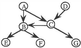
In this paper, we use the network proposed by Smets (1993 ) for the propagation of beliefs. Graphically, the network is a directed acyclic graph (dag) as defined in Pearl (1988) for the Bayesian networks, shown in Figure 1. A gr ap h G = (M, E), where Mare the finite sets of nodes and E are the sets of edges, is said to b e a dag when there is no path n 1 n2 . . . nk such that (n i , ni+l)e E (l<i::;k - 1) and nt=nk. However, the conditional beliefs are defined in a different way. In our network, each edge represents a conditional relation between the two nodes it connects. In order to d i s t i ng u i s h these two kinds of networks, we call ours ENC, which means an �vidential network with £Onditional be li e f functions. We also assume that, for each c o n d i ti on al belief function for Y given X, a ll we know about Y given X is initially represented by the set { b e l y ( . l x j ) : XiE E>x}. For example, in Figure 1, edge (A, B) r e p r e se n t s a conditional belief function for the node B g i v e n A, r e p res e nt ed by bel B (.Iai): a i E E>A
One main object of reasoning process in ev i de nt i a l network is to c o m p u t e the marginal distributions for some variables. We use BELx to denote the ma r g i n a l for variable X, b e l o x the a priori belief for X. Due to the DRC a n d the GBT, given two variables X andY, and the conditional b e l i e f bely(.lx i ): xjE E>x, we could compute and store bely(.lx): xt;;;;E> X and b e l x ( . l y ) : yt;;;;E>y i n the preprocess, which might be useful for speeding up the c o m p utati o n in the propagation. Now, we are ready to give the inference algorithm: Given an ENC r ep r e se n t ed by G=(M,E)
� p ro p a ga t i ng beliefs in polytrees, i.e., there i s only one (undirected) path between any of two nodes in the network:
Propagation algorithm can be regarded as a message passing scheme: for each node X in the network, its marginal BELx is computed by combining all the messages from its neighbors Nx={Y(E M)I(X, Y)E E or (Y, X)EE) and its own a p r i o ri belief belox- i.e.,
BELx= belox 0 (0 (MY--tX I Ye Nx}) (9) where the message My --tX is a belief function on X, so it can be represented by bely--tx or mY--tX· and is computed by: for any xt;;;;E>x
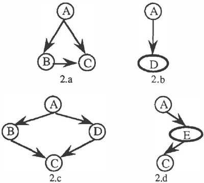
Case 2: If th er e exist any undirected loops in the network, then some nodes needed to be merged to m ak e the network acyclic, resulting in a new polytree G'=(M', E'), where some nodes in G' might be a subset of the nodes i n G, we call this kind of node a merged node. For any merged node v in G', there might be a belief function Rv o b ta in e d by the ballooning extension of condit i on al beliefs. Figure 2 illust r a t e s two examples for this process:
In Figure 2.a, the loop is absorbed by merging nodes B and C, the resulting graph is s h o w n in 2.b where D={B, C}, and new conditional belief function belo(.la i ) is obtained by combining belB(.la i ) and belc(.la i ) on the space E>o=E>Buc: 'v'aiE E>A, dt;;;;E>o ,
Obviously, belo(dlaj) is normalized iff bels(.ia i ) and belc(.ia i ) are normalized since the subset b i{B , Cl n c i(B,CJ can never be an empty set. Moreover, the conditional belief function between B and C becomes Ro in Figure 2.b obtained by the ballooning extension of bels(.iq) applying eq. (8). Thus Ro is a belief function on E>D.
Figure 2.c is another example of ENC with a loop. In this case, we merge B and D, resulting in the graph shown in 2.d, where E= {B, D). bel E (.Ia i ) is obtained by combining bels(.la i ) and belD(.ia i ) on E>E=E>auo using eq. (11). As for belc(.ie): ecE>E, we compute it for three cases:
2) for e<;:SE, if e can be represented by bxd, where bcE>s. dc El o .
where mc(.ib) and mc(.ld) are obtained from mc(.lbi) and mc(.idj) respectively by applying the DRC as shown in equations (4);
3) for any other e<;:E>E. we first construct a conditional belief function belcuo(.ib i ) from mc(.ib i ) such that
= mc(clb i )
mcuo(slbi)
where s = c1'{ C , Dl n ((enb/E).I.(D))t[C,DJ,Iet bel � uo be the belief function resulting from the b a l loon i n g extension of mc(.ld i ). then
Alternatively, belc(.le): ecE>E can be computed by first com b i ni n g the ballooning ex t e n si o n s of the two conditional beliefs belc(.lb i ) and belc(.ldj) on t h e space E>suc and E>cuo. then using equation (7) to transfer the resulting belief in a conditional form belc(.le):ecE>E and belE(.ic):q;;;Elc. However, this takes more space for the computation.
Since there is no direct relation be t w e en Band D, RE is a vacuous belief function.
After transforming the network to an acyclic one, we then use a similar algorithm in easel for the propagation: Suppose each node X in G' is a subset and has a R x . Thus, for any non-merged node, it is a singleton, and R x is a vacuous belief function. Then the computation is as following: for any node A={Xt, . .. , X t l in G',
the message My �A f ro m Y to A is computed by: for Y={Yt, ... Ynl.
Although the above representation and propagation algorithm are for the networks which only have binary relations between the nodes, it could be generalized to the case where relations are for any number of nodes. In the rest of this section, we will show some special cases where using ENC can reduce the computation.
Definition 9: Let X, Y be two nodes in ENC, where Elx={x1, .. , x p } , E>y={y1, .. ,yq}. Suppose there is an edge (X, Y) representing a conditional belief for Y given X: bely(.lxj): X i E Bx such that m(9ylxj)<1 for i::d, .. . ,t(<p) and m(Elylxj)::::l for j ::::t + l, .. ,p. We say the elements X i 's (i:;t) are relevant to Y and xj's (t<j:;p)irrelevant toY.
This kind of relationship exists commonly in the diagnosis problems and rule-based systems. In Example 1, we say that a is relevant to B, but -a irrelevant to B. Intuitively, it means that given some knowledge on a, we can induce knowledge about B, but no matter what we know about -a, we can't induce any knowledge about B. Thus we say -a is irrelevant to B.
Lemma 7: Given two variables X, Y and the conditional bel on Y given X, suppose <l>={X t +l· .. , x p } is irrelevant to Y. Then for any subset S of E>x. if Sn<t>=t:0, then my(E>yiS)=l.
Proof: The result can be derived directly by applying the GBT. QED
Lemma 8: Given two variables X, Y and a conditional bel on Y given X, suppose <l>= { X t + 1 , .. , x p } is irrelevant to Y. Assume we have some belief belo o n Y, by theorem 1-3, we can compute the belief of X. If mx(S)=t:O, then S;:;2<l>.
Proof: From lemma 7 we have, \fxcE>x, if xn<I>=t:0, my(Elylx)::::l, i.e., pl y (ylx)=1 for \fycE>v. Then, by
equations (5) and (6), pl x (xly)=pl y (ylx)=l for such x. Thus by equation (7), we have
Therefore, VS<;;;8 x , if mx(S);tO, S should contain any element o f ct>, i.e. S::::::1 ct> . QED
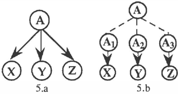
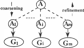
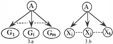
From lemma 7 & 8, we can simplify the computation for some special cases of ENC, shown in Figure 3, where in 3.a, G i is a group (set) of variables and suppose some elements cl>i of A are irrelevant to each variable X i . Figure 3.b shows detail in each G i . To describe the computation, let's begin by recalling the concept of partition:
Definition 10: Let 8 = (El 1, ... , El p ) be a frame of discernment. A set 'f' e of subsets of 8 is a partition of e if the elements in 'f' e are all non-empty and disjoint an d their union i s e. We also call 'f'e a coarsening of 8 and e a refinement of 'f'e.
From the definition, we have VEliE e, ::Jx j E f'e which is a mapping of ei · We denote such mapping by A(Si)=xj. VEJ<;;;8, A(S)=(A(Si)IEliE 8). Let bel1 be a belief function on e, then the belief bel2 on 'f' e induced by bel�o sa y , by coarsening, is obtained by: Vx<;;;f' e.
Let bel2 be a belief function on 'f' e. bel1 on e induced by bel2, say, by refinement, is obtained by: El<;;;8, x<;;;'f'e, m(El) = m(x) (14.2)
where El = u(El' I A(El') = x}
Given a network as shown in Figure 3, we can represent it as a two-level structure shown in Figure 4. Each A i has a frame 8A j which is a partition of 9A SUCh that \f a k E 9A, A(ak)=S i if akE(n{<I>j I Xj<;;;;;Gi}), o th e rw i se A(�)={�}=ak. In fact, S i =n{cl>j I Xj!;;;Gi}. Each IAi�Gil part can be regarded as a local sub-network, and the belief functions passed between A and A i are performed by refinement and coarsening between the two frames. Let's look at the following example:
Example 3; Suppose we have 4 variables in the network (shown in Figure S.a): A, X, Y and Z. Their frames are: 8A = (at, a2, a3, 34, as}, ex= 8y = 8z = { +, -}. The relations among them are represented by conditional belief functions in Table 3.
Table 3: Conditional belief functions for example 3
| a t a s | 34 | a2 | a3 | a t a 3 | a 2 | <14 | a s | ||
| + | . 9 | .7 | 0 | 0 0 | + 0 | .7 | .2 | .4 | 0 |
| 0 | .3 | 0 | 0 0 | 0 | .3 | .6 | .1 | 0 | |
| e | . t | 0 | 1 | 1 | e 1 | 0 |
1
.2
.5
1
| a t | a 2 | a3 | 34 | a s | |
|---|---|---|---|---|---|
| + | 0 | 0 | 0 | .6 | .9 |
| 0 | 0 | 0 | .3 | 0 | |
| e | 1 | I | I |
1
. I
.1
Now suppose that we have some observation about X and Z: mox( ( + })=.8, mox(6x)=.2; moz( ( -})= 1. To compute the marginal for A, if we use the joint belief for the relation A and X, then the combination is performed on the product space ElAux and 8Auz; if we use the conditional belief represented in the above tables, the computation is performed on the frame eA, which is more efficient. Moreover, if we use the result of lemma 8, the computation can be simplified further. The following steps illustrate such computation:
- transform the network in S.a to the network shown in Figure 5 .b where each 8 Ai is a partition of 9 A:
9At"'{al, 32, st) (st={a3,a4,a5}) 8A 2 ={a2, 3J, a4, s2}, and eA3={a4, as, s 3 }. belx(.laj): aie eA1 is obtained from belx(.laj): ajeeA. belx(.lst): StE8A1 is obtained by applying the DRC, Symmetrically, we can get the other two conditional beliefs. The resulting conditional beliefs are shown in Table 4:
- Using the DRC to compute be l A 1( . 1x) a n d be i A 3 ( . 1 z ) .
- Using Theorem 2-3 to compute belA i : i"'1,2,3. belA2 is vacuous by lemma 3; mA1((al, stJ)=.24, mA1(9A1)"'.76; and mA3( {SJ})=.54, mA3({a4,SJ})=.36, mA3((as,S3 })=.06, mA3(8A3)=. 0 4.
- compute the above two beliefs On the frame e A by refinement and combine them, we get our desired result.
| mx (xlai): 8iESA t | my(ylaj):aiE 9Az | mz(zlaj):aiE 8AJ |
| al a2 St | 32 33 a4 S2 | 34 as SJ |
| + .9 .7 0 | + .7 .2 .4 0 | + .6 .9 0 |
| 0 .3 0 | - .3 .6 .1 0 | - .3 0 0 |
| e 0 1 | e 0 .2 .5 1 | e .1 .1 I |
.1
Obviously, this computation is more efficient since in Step 2 and 3, the computation is taken on the frame e Aj which is smaller than 9A.
Moreover, if the network has the properties defined as below, we can also simplify the computation for each sub-network shown in Figure 3.b.
Definition 11: Let X, Y and A be three nodes in an ENC, where ex"'(x}, ... ,x p }, Sy=(yJ, ... ,yq) and SA= {a1, . .. ,at}. Suppose we have belx(.lai) and bely(.lai) for a i E eA. Let <I>x, cl>y�eA be the sets of irrelevant elements for X and Y respectively. <t>x;e0, <lly;e0. X and Y are unrelated through A, denoted by u(X,Y ,A), if <llx and <lly satisfy:
- (I) <l>x n cl>y -t:. 0 ; or
(2)ct>xn<l>y=0, <l> x u <l> y = S A , belx(.l <i> x) or bely(.l <i>y) obtained from belx(l.a i ) or bely(.la i ) by the DRC is vacuous.
This relation can also be extended to the two disjoint subsets, where <l>A: A�U is defined as: <t>A = n ( <t>x I X e A ) .
Lemma 9: Let X, Y and A be defined as in definition 11. Suppose we have belx(.laj) and bely(.laj) for aiESA, but no a priori belief on A. Now suppose we have observations about X, then BEL y is vacuous if X a n d Y are umelated.
Proof: This can be proved by applying the r e s u l ts of lemma 7 and 8. QED
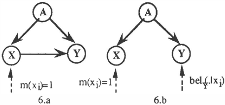
Now let's consider the computation for the network shown in Figure 6.a. Let X, Y, A, <l>x and <l>y be defined as in definition 11. Assume X and Y are binary variables. Suppose we have conditional beliefs for X and for Y given each element of 8A, u(X,Y,A) andci>x n ci>y = 0 , the conditional belief for Y given X bely(.lx i ): i=1,2 is such that bely(.IE> A) obtained from bely(.lx i ) is vacuous. If all the a prori beliefs for the variables are vacuous, the propagation result would be vacuous. Now suppose we have observations about X: X=Xj, then the network in 6.a is equivalent to the one shown in 6.b (Proofs can be found in (Xu and Smets 1994)).
The computation of Figure 6.b is obvious by applying the DRC and the GBT. Let mAixi denote the resulting bel i ef for A. Furthermore, if the observation about X is any kind of belief function, we can compute BEL A for A as follows: VaceA,
If there exists some a priori belief for A: beloA. then the marginal for A is computed by the combination of the above resulting belief function and belo A ·
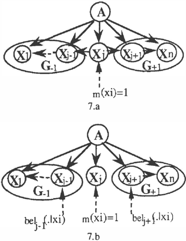
This method avoids the computation on the frame of 8 AuXuY for the case where the conditional belief is represented in joint form and avoids merging nodes to compute bel(alx,y) and bel(,;,y) as described in the beginning of the section, thus it simplifies the computation for such kind of network. This method can also be extended for the case shown in Figure 7.a, under the condition that u(G.loG+tu{Xj},A), u(G+l>G-tu{Xj}, A) and the intersection of the relevant elements of each pair of G_1, G+1 and Xj is empty. The network in 7.a is equivalent to the one in 7.b (Proofs can be found in (Xu and Smets 1994)). If Xj's inside G have similar relationship, we can iteratively use the scheme described above to compute the marginal for A.
5. CONCLUSIONS
We have presented an ev i d e n tia l network (ENC) w h i c h uses conditional belief functions for the knowledge representation and reasoning. In t h e paper, we have � � mpare? some relations between the r e p r e s e n tat i o n by JOmt belief and by c o ndi t i on a l belief and we h a v e found that the conditional form is more natural and it takes less space. We also pr o v id e a n a l g o r i t h m for r easo nin g in ENCs. The presented a l g o r i t hm of reasoning is only for t he network where all the relations are binary, t h e extension of the algorithm to a general case will be studied in the f ut ur e w o rk. A l though we h a v e compared the computational complexity of ENC and the network using joint beliefs in a general case, we h a v e shown that in s o m e special cases, the computation of ENC can be � i i_D pl i f i �d and is more e ff i c i e n t than the network us in g JOmt b e l i e f s . The advantage of simplified computation in suc h networks can be shown in the example abstracted from (Xu et al. 1993).
Acknowledgments
T h i � research work has been p a r t i a l ly supported by t h e Acuon d e Recherches Concertees BELON funded by a grant from t h e Communaute Fran�aise de Belgique a n d the ESPRIT III, Basic research P ro je c t Action 6156 (DRUMS II) funded by a grant from the Commission of the European Communities. The authors are grateful to anonymous r e v i e w e rs for their comments and suggestions. The first author w o ul d like to ac k n o w l edg e the support by a grant of IRIDIA, Universite libre de Bruxelles.
References
Cano J., D elga d o M., and Moral S. "An Axiomatic Framework for Propagating Uncertainty i n Directed Acyclic Networks" /JAR, 8:253-280, 1993.
Dubios D. and Pr ad e H. "A set theoretical view of belief functions" I n t . J. Gen. Systems, 12:193-226, 1986.
Pearl J., Probabilistic Reasoning in Intelligent Systems: Networks of Plausible Inference, Los Altos, CA, Morgan K a u f m ann , 19 88 .
Shafer G., A Mathematical Theory of Evidence Princeton University Press, 1976.
Shafer G. an d Shenoy P. P. "Local Co m p u tat i o n in Hypertrees" Working Paper No. 201, School of Bu s iness , University of Kansas, Lawrence, KS, 1988.
Shenoy P. P. and Shafer G. "Axioms for p ro b a b i l i t y and belief functions propagation", Uncertainty in Artificial Intelligence 4, (Shachter R. D., Levitt T. S., Kanal L. N. and Lemmer J. F. eds.), North-Holland, A mste r d am , 159-198, 1990.
Shenoy P. P., "Valuation-Based S y s t e ms : A framework fo r managing uncertainty in expert s y s t em s " Fussy logic for the Management of Uncertainty (L.A. Zadeh a n d J. Kacprzyk eds.), John Wi l ey & Sons, NewYork. pp. 8 3 -1 04 , 1992.
Shenoy P. P., "Valuation Networks and Conditional Independence" Proc. 9th Uncertainty in AI (M. P. Wellman et. al. ed s .) , San Mateo, C al i f . : Morgan Kaufmann, pp.l91 -199, 1993 .
Smets Ph. "Un modele mathematico-statistique s i m ulant le processus du diagnostic medical", Doctoral dissertation, Universite libre de Bru x e l l e s , 1978.Smets Ph., "Belief Functions" Non S t{JJ'!(brd Logics for Automated Reasoning ( S m et s Ph., Mamdani A., Dubois D. and Prade H. eds.), A c a d em i c Press, London, 253-286, 1988.
Smets Ph. "The combination of evidence of the transferable belief model" IEEE-Pattern Analysis and Machine Intelligence, 12:447-458, 1990.
Smets Ph., "Belief F un c t i o ns : the D i s ju n c t i v e Rule of Combination and the Generalized B a ye s i an Theorem" /JAR, Vol. 9, No. 1 pp. 1-35, 1993.
Xu H., Hsia Y. an d Smets Ph., "A belief f u nc t i o n bas ed d e c i s ion s u p p o r t s y s t e m " Proc. 9th Uncertainty in AI (M. P. Wellman et. al. eds.), San Mateo, Calif.: Morgan Kaufmann, pp.535-542, 1993.
Xu H. and Smets Ph., "Evidential reasoning with conditional belief functions" Technical Report TR/IRIDIA/94-5, U n iv e r s i te libre de Bruxelles, Be lgium , 1994.